↗ OpenReview ↗ NeurIPS Homepage ↗ Chat
TL;DR#
Current zero-shot image denoising methods often produce blurry results or require significant computation time. This is because they typically train new networks from scratch for each noisy image, limiting the information available for training and affecting quality/speed. Existing methods also struggle with generalizing across different noise types.
The paper introduces Masked Pre-train then Iterative fill (MPI), a new zero-shot denoising approach. MPI first pre-trains a model on a massive dataset of natural images using a masking strategy. Then, it uses this pre-trained model to iteratively refine a single noisy image, focusing on masked regions to minimize the gap between pre-training and inference. This method significantly improves denoising quality and speed, outperforming existing zero-shot methods while demonstrating robust generalization to different noise types and even medical images.
Key Takeaways#
Why does it matter?#
This paper is crucial for researchers in image processing and computer vision due to its introduction of a novel zero-shot denoising paradigm. The universal applicability across diverse noise types and image modalities, along with the significant reduction in inference time, makes it highly relevant to current research trends and opens new avenues for practical applications. Its innovative use of masked pre-training offers a promising direction for future research in zero-shot learning and image restoration.
Visual Insights#

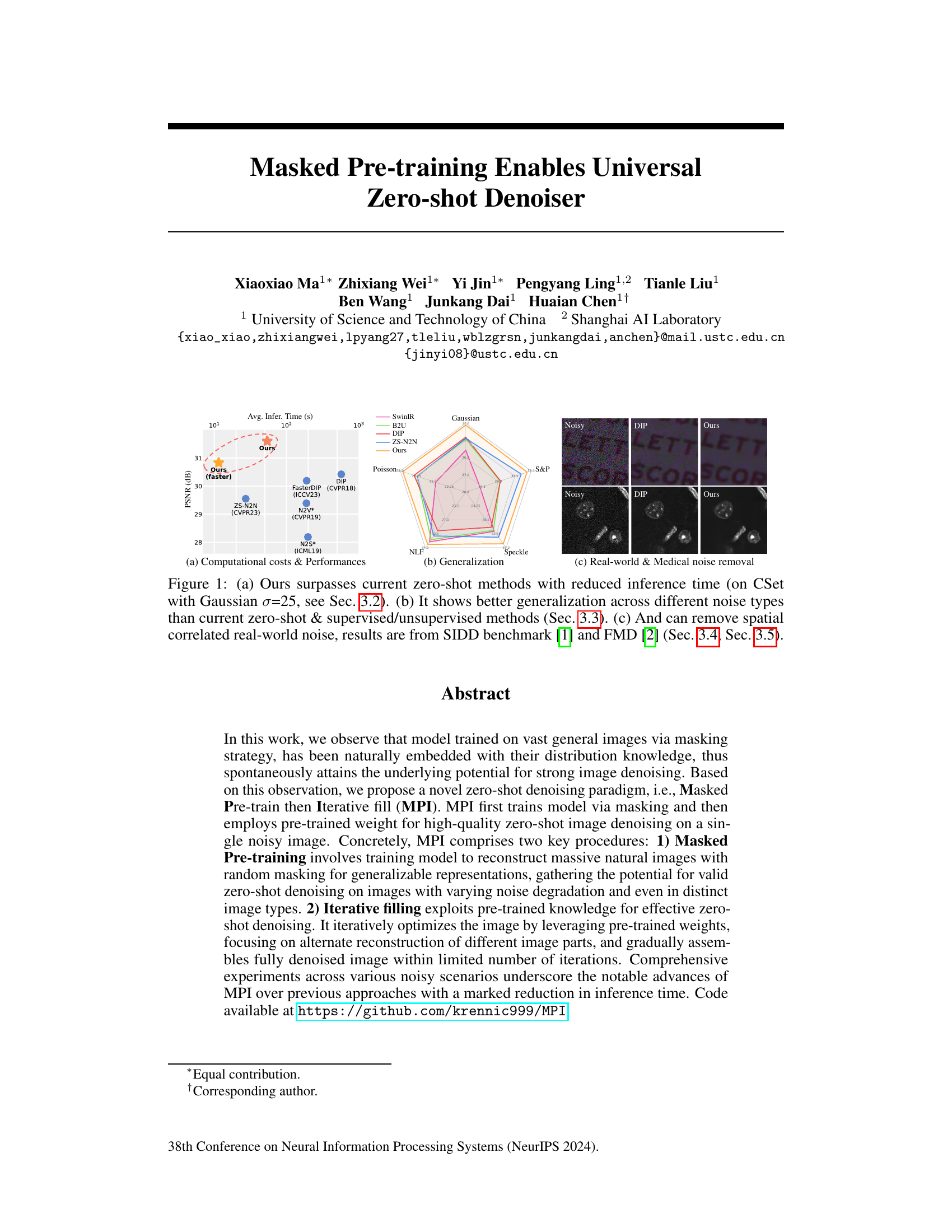
This figure demonstrates the superior performance of the proposed method (Ours) compared to existing state-of-the-art zero-shot and supervised/unsupervised image denoising methods. Panel (a) showcases a significant reduction in inference time while maintaining competitive performance with respect to Peak Signal-to-Noise Ratio (PSNR). Panel (b) highlights improved generalization across diverse noise types. Lastly, panel (c) visually presents the effectiveness of the method in removing real-world and medical image noise, demonstrating its superior performance compared to existing methods.

This table presents a quantitative comparison of different image denoising methods on three datasets (CSet, McMaster, and CBSD) for Gaussian noise removal. The comparison is done across different noise levels (σ = 10, 25, 50). The results are presented in terms of PSNR and SSIM values, with the best results highlighted and the second-best underlined. The table also includes the average inference time for each method. Supplementary materials provide similar results for Poisson noise removal.
In-depth insights#
Masked Pre-train#
The Masked Pre-train phase is critical to the success of the MPI (Masked Pre-train then Iterative fill) model. It leverages masked image modeling on a large dataset of natural images (like ImageNet) to learn robust and generalizable image representations. Random masking strategically obscures portions of the images, forcing the model to reconstruct the missing parts based on contextual information. This process effectively encodes the inherent structure and statistical properties of natural images into the model’s weights. The resulting pre-trained model, therefore, isn’t just a denoiser trained on specific noise patterns, but rather possesses a powerful capacity for zero-shot generalization. This pre-training phase is what allows the model to handle unseen noise types effectively during the subsequent iterative filling steps. The choice of masking strategy, the size of the dataset, and the training procedure all play important roles in ensuring that the model effectively learns the underlying structure of the image, which then provides a strong basis for later zero-shot inference. It’s a key innovation, differentiating MPI from traditional zero-shot denoising methods that train entirely from scratch on a single noisy image.
Iterative Filling#
The proposed method, Masked Pre-train then Iterative Fill (MPI), innovatively uses an iterative refinement strategy called “Iterative Filling” for zero-shot image denoising. Instead of training a new model for each noisy image, MPI leverages pre-trained weights from a model trained on a massive dataset of natural images using a masked image modeling approach. This pre-trained model already implicitly possesses knowledge about image structures and distributions, providing a strong foundation for effective denoising. The iterative filling process progressively refines the noisy image through iterative optimization, focusing on masked regions in each step and gradually assembling a complete denoised image. This strategy is particularly effective as it avoids overfitting to the specific noise characteristics of a single noisy image while still exploiting the power of pre-trained knowledge for high-quality results. The iterative approach makes the method more efficient than traditional zero-shot methods that train a new network from scratch for every image. The combination of pre-training and iterative refinement is key to achieving both high performance and significantly reduced inference time.
Real-world Noise#
The section on real-world noise in this research paper is crucial because it addresses the limitations of existing denoising methods that primarily focus on synthetic noise. Real-world noise is significantly more complex, exhibiting strong spatial correlations and varying intensity levels. The authors acknowledge that simply applying masking strategies designed for synthetic noise is insufficient for effectively handling real-world scenarios. Consequently, they propose incorporating downsampling to reduce spatial correlations, along with a larger masking ratio to better capture the characteristics of real-world noise patterns. This approach showcases the generalizability and robustness of their proposed masked pre-training method, demonstrating its effectiveness in scenarios that go beyond the constraints of laboratory-generated datasets. The results on real-world datasets, such as SIDD and PolyU, further highlight this method’s capabilities. This is a key strength of the paper as it bridges the gap between theoretical findings using synthetic datasets and practical applications using real images with varied noise types.
Generalization Limits#
The heading ‘Generalization Limits’ in a research paper would explore the boundaries of a model’s ability to perform well on unseen data. A thoughtful analysis would delve into factors limiting generalization, such as the size and diversity of the training dataset, the model’s architecture and capacity, and the nature of the noise or variations present in the data. The discussion might include a comparison of performance on training data versus unseen data, possibly quantified by metrics like generalization gap. It would be crucial to identify specific types of noise or data distributions where the model underperforms, along with an exploration of the reasons why. For instance, a model trained on Gaussian noise might fail to generalize to real-world noise with complex spatial correlations. A strong analysis would also discuss the extent to which the model’s limitations are inherent to the task itself or whether they result from specific design choices. Ultimately, the section on ‘Generalization Limits’ would reveal valuable insights into the robustness and applicability of the presented research.
Future Directions#
Future research directions for masked pre-training in zero-shot image denoising could explore more sophisticated masking strategies, moving beyond simple random masking to incorporate spatial and frequency information. This might involve adaptive masking that adjusts the masking ratio based on image content complexity or noise characteristics. Furthermore, exploring different pre-training datasets beyond ImageNet, perhaps incorporating specialized datasets for specific noise types or image modalities, could improve performance on less-represented domains. Investigating alternative optimization methods during the iterative filling stage, potentially employing techniques from diffusion models or other advanced optimization frameworks, could yield higher quality denoised images. Finally, a thorough investigation into the generalization capabilities of the approach, evaluating its performance on a wider range of unseen noise types and image modalities, is crucial for practical application. Specifically, applying the proposed method to real-world challenging scenarios, such as medical imaging or low-light photography, will offer valuable insights and potential improvements.
More visual insights#
More on figures

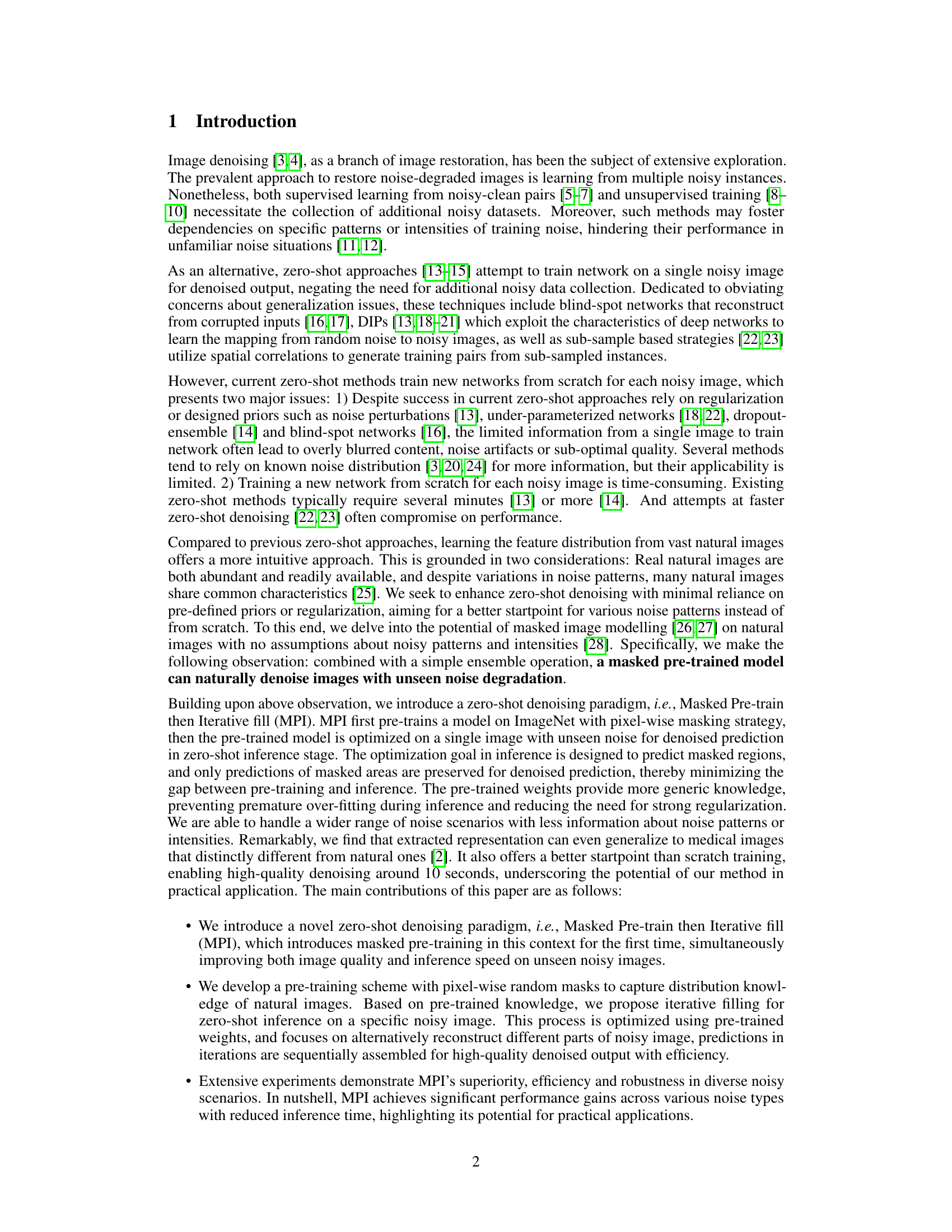
The figure shows the results of applying a model trained on ImageNet with 70% pixel-wise masking to a noisy image. The ‘Directly ensemble’ column shows the result of simply averaging predictions from the pre-trained model, demonstrating a basic level of denoising. The ‘+Zero-shot Optim.’ column, on the other hand, shows the result of applying iterative filling which further improves upon the quality of the denoised image. This illustrates the effectiveness of the proposed iterative filling optimization step for zero-shot denoising.
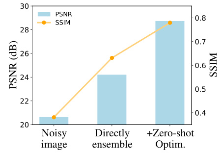
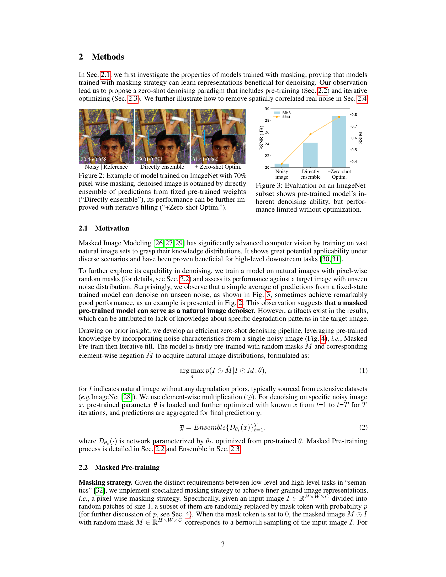
The figure shows the PSNR and SSIM values for a noisy image, a denoised image obtained by directly averaging the predictions from a pre-trained model, and a denoised image obtained by further optimizing the pre-trained model using an iterative filling method. The iterative filling method significantly improves the PSNR and SSIM values, demonstrating its effectiveness in enhancing denoising performance.
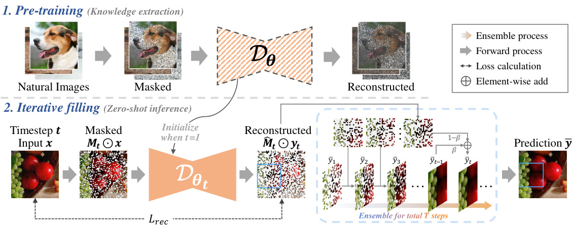
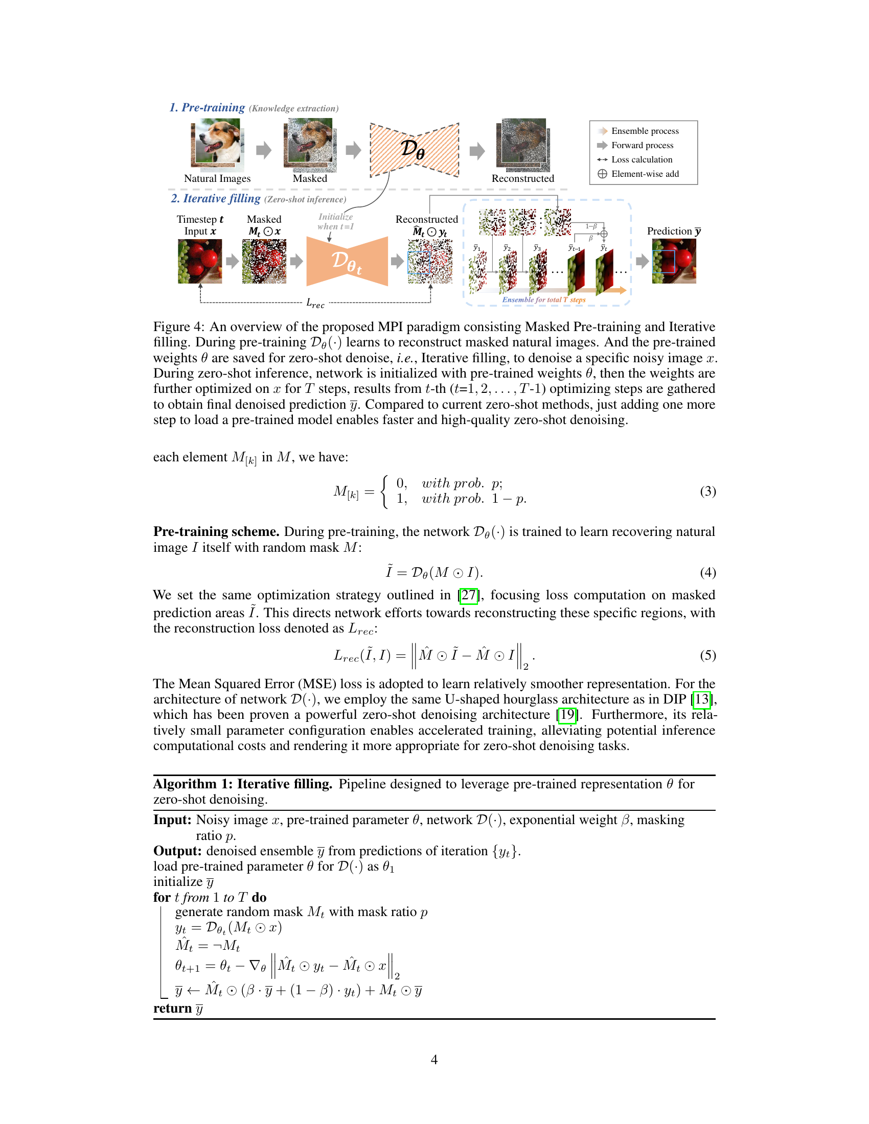
This figure illustrates the Masked Pre-train then Iterative fill (MPI) paradigm. It shows the two main stages: 1) Masked Pre-training where a model learns to reconstruct masked natural images, extracting general knowledge about image distributions. 2) Iterative Filling, a zero-shot inference process where the pre-trained model is fine-tuned on a single noisy image to iteratively refine its denoising capabilities. The iterative process involves masked predictions, where only predictions for masked regions are retained to avoid overfitting and achieve efficient denoising in a limited number of iterations. The final denoised image is created by combining predictions across all the iterations.

This figure demonstrates the superiority of the proposed method (Ours) over existing zero-shot and supervised/unsupervised image denoising methods. Panel (a) shows a comparison of computational cost and performance, highlighting the faster inference time of the proposed method. Panel (b) showcases its better generalization across various noise types. Finally, panel (c) illustrates its ability to effectively denoise real-world and medical images.

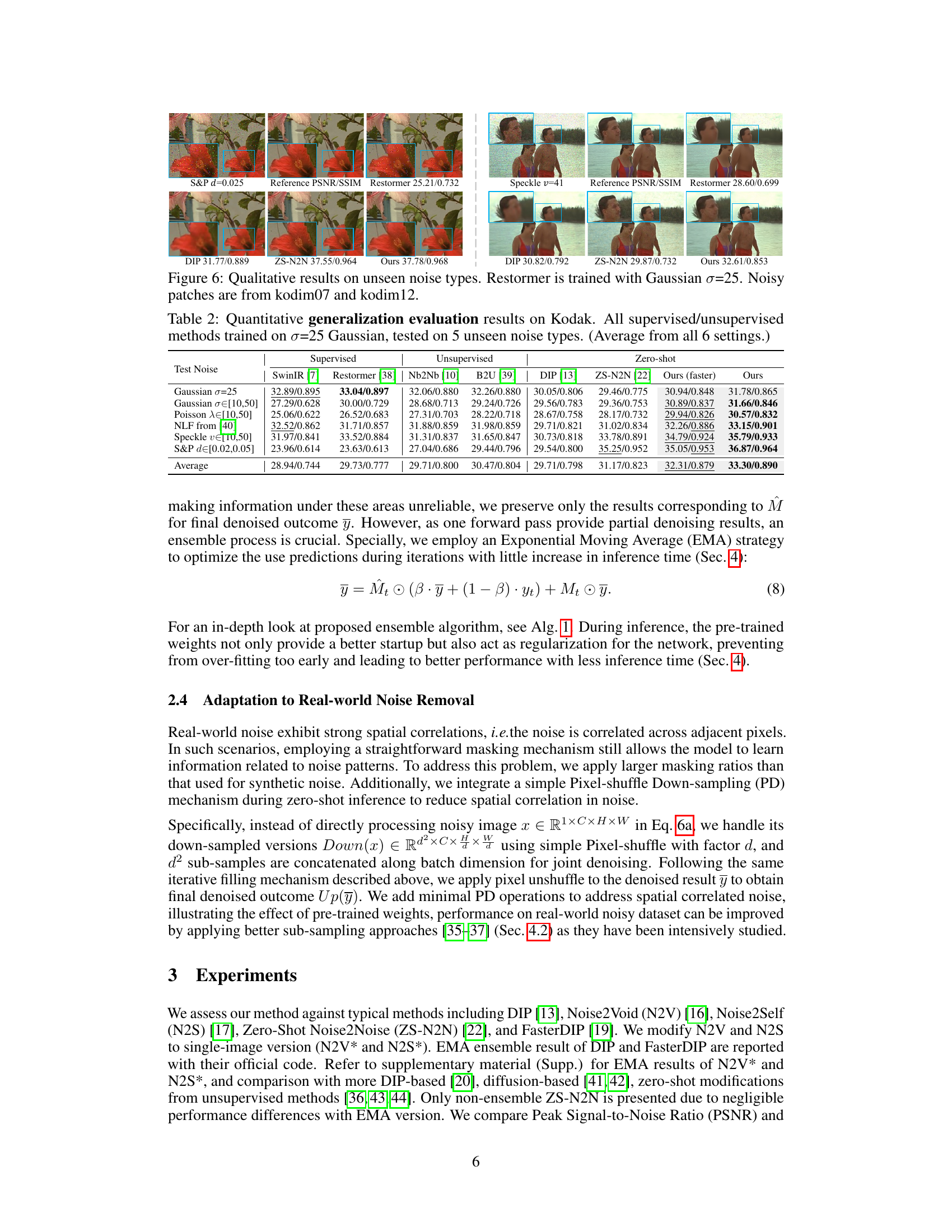
This figure shows qualitative comparisons of denoising results on unseen noise types (salt & pepper and speckle noise). The results of the proposed method (MPI) are compared against several other methods including DIP, ZS-N2N, and Restormer. Restormer, a model trained on Gaussian noise, serves as a baseline for comparison. The figure highlights the superiority of the proposed MPI method in handling these different unseen noise types, producing images with noticeably improved visual quality and fewer artifacts.
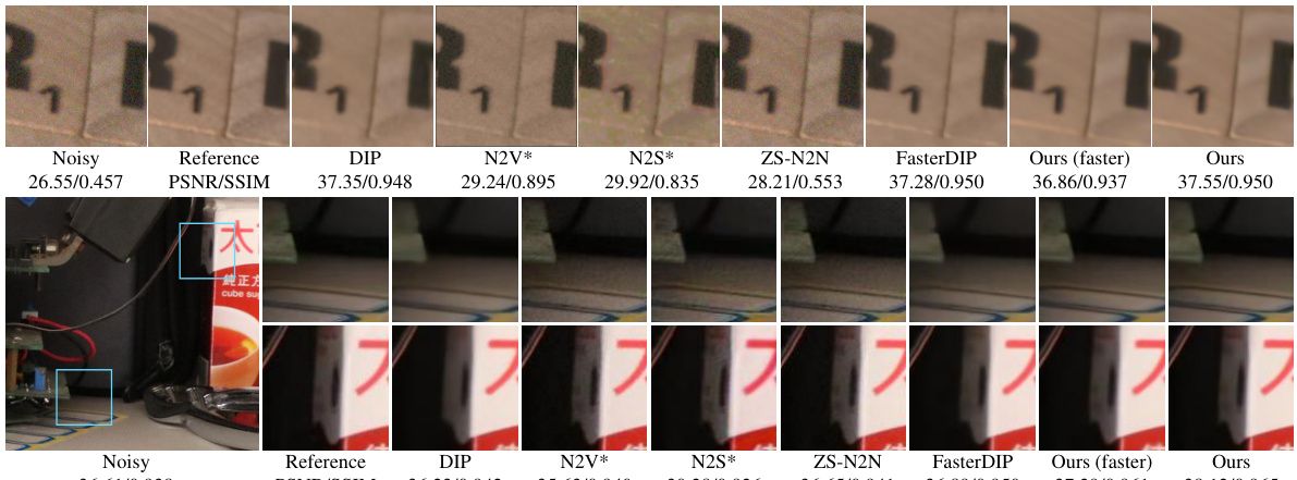
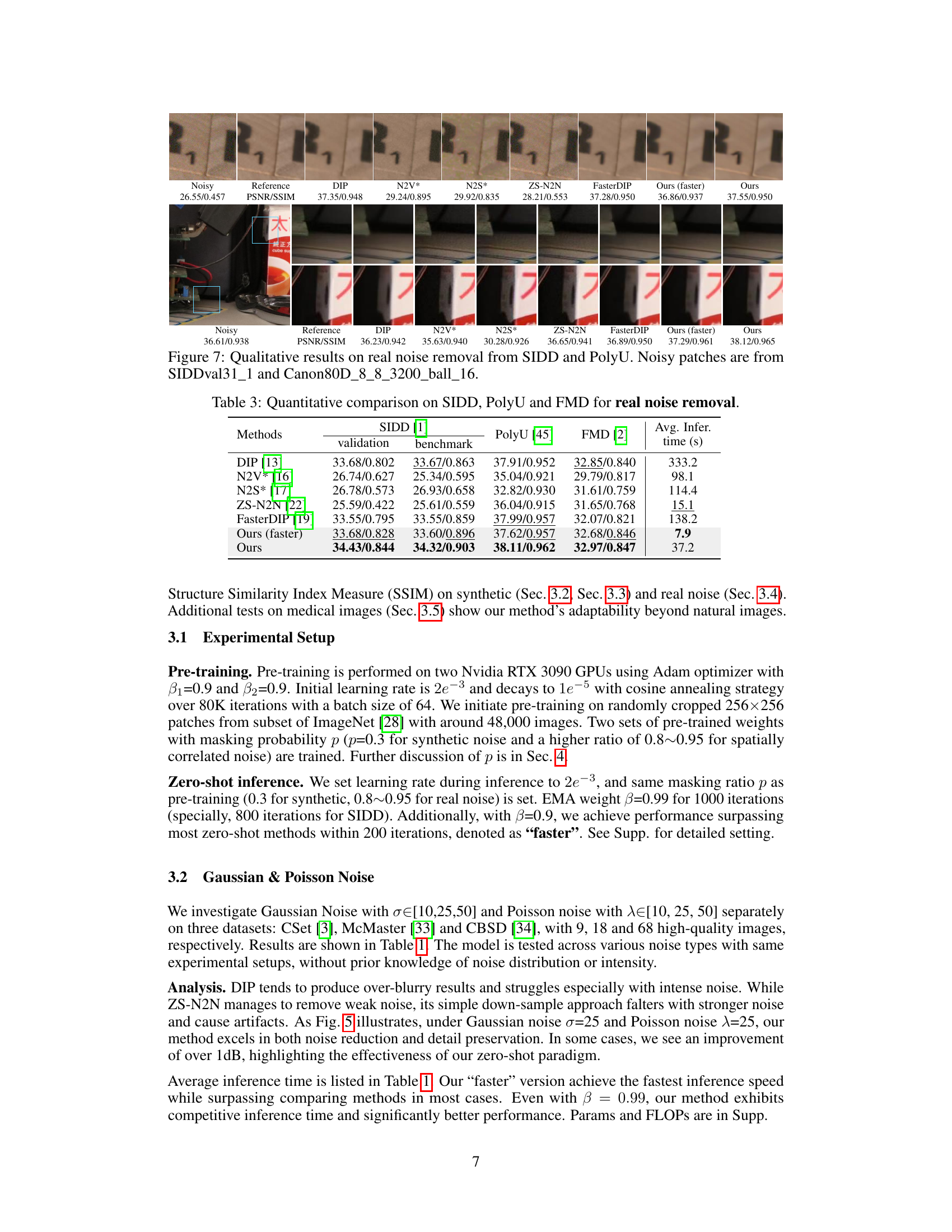
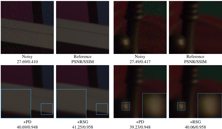
This figure shows the qualitative results of the proposed method on real-world noisy images from two datasets: SIDD and PolyU. The results are compared against several other state-of-the-art denoising methods (DIP, N2V*, N2S*, ZS-N2N, FasterDIP). The figure showcases the visual improvements achieved by the proposed method, particularly in terms of detail preservation and noise reduction. The PSNR/SSIM values are provided below each image, which quantifies the performance gains.

This figure shows that the pre-trained model generalizes better to unseen noise types compared to a model trained from scratch. The results show that the pre-trained model is able to denoise images with unseen noise better than a model trained from scratch, even when the content of the image is different from the images used in pre-training. This suggests that the pre-trained model has learned a more general representation of images that is able to handle unseen noise better than a model trained only on seen noise. The result indicates the model trained on ImageNet with 70% pixel-wise masking, The denoised images are obtained by directly ensemble of predictions from fixed pre-trained weights. Its performance can be further improved with iterative filling.
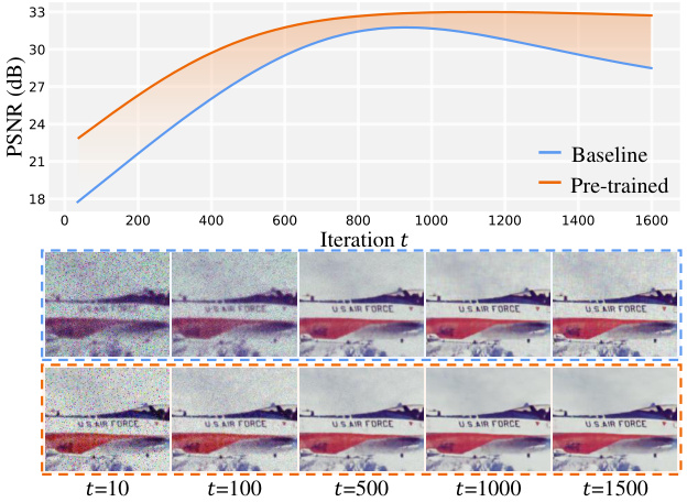
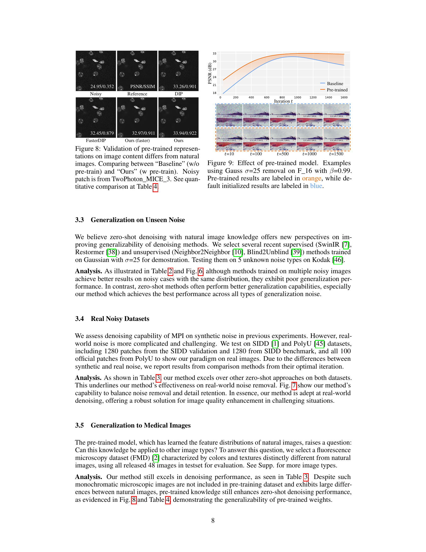
This figure shows the effect of using a pre-trained model for denoising. It presents a comparison of denoising results on an image with Gaussian noise (σ=25) at different iterations (t=10, 100, 500, 1000, 1500) using both pre-trained weights (orange) and weights initialized from scratch (blue). The results visually demonstrate that the pre-trained model leads to better denoising performance, even at earlier iterations.
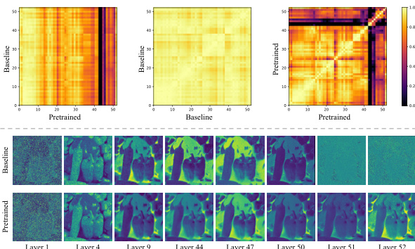
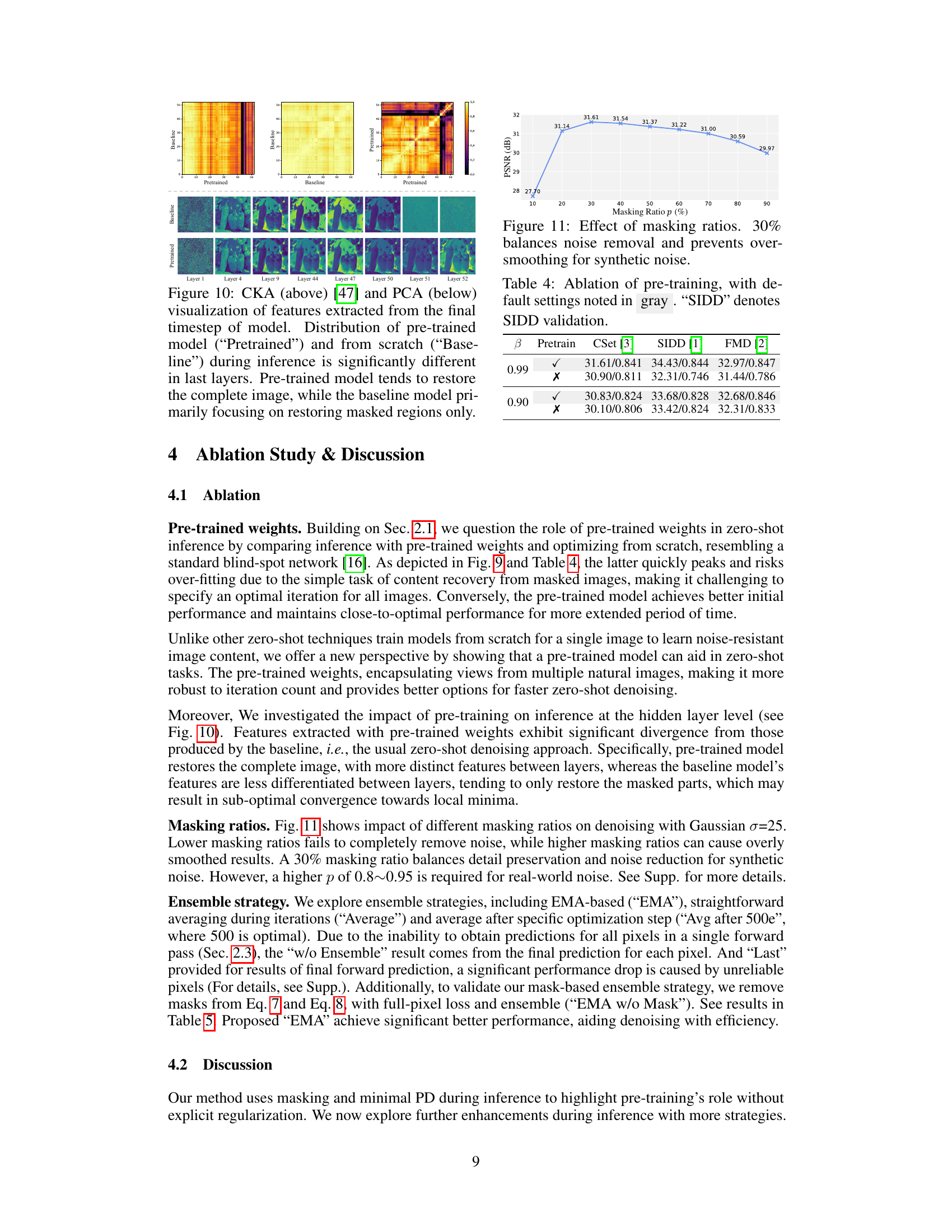
This figure shows the visualization of features extracted from different layers of the model during inference. The top row shows the CKA and PCA analysis of the features, which reveals that the pre-trained model and the model trained from scratch have significantly different feature distributions in the last layers. The bottom row shows the feature maps from selected layers of the pre-trained model and the model trained from scratch. This comparison shows that the pre-trained model tends to restore the complete image, while the model trained from scratch focuses primarily on restoring the masked regions.
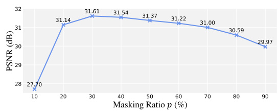
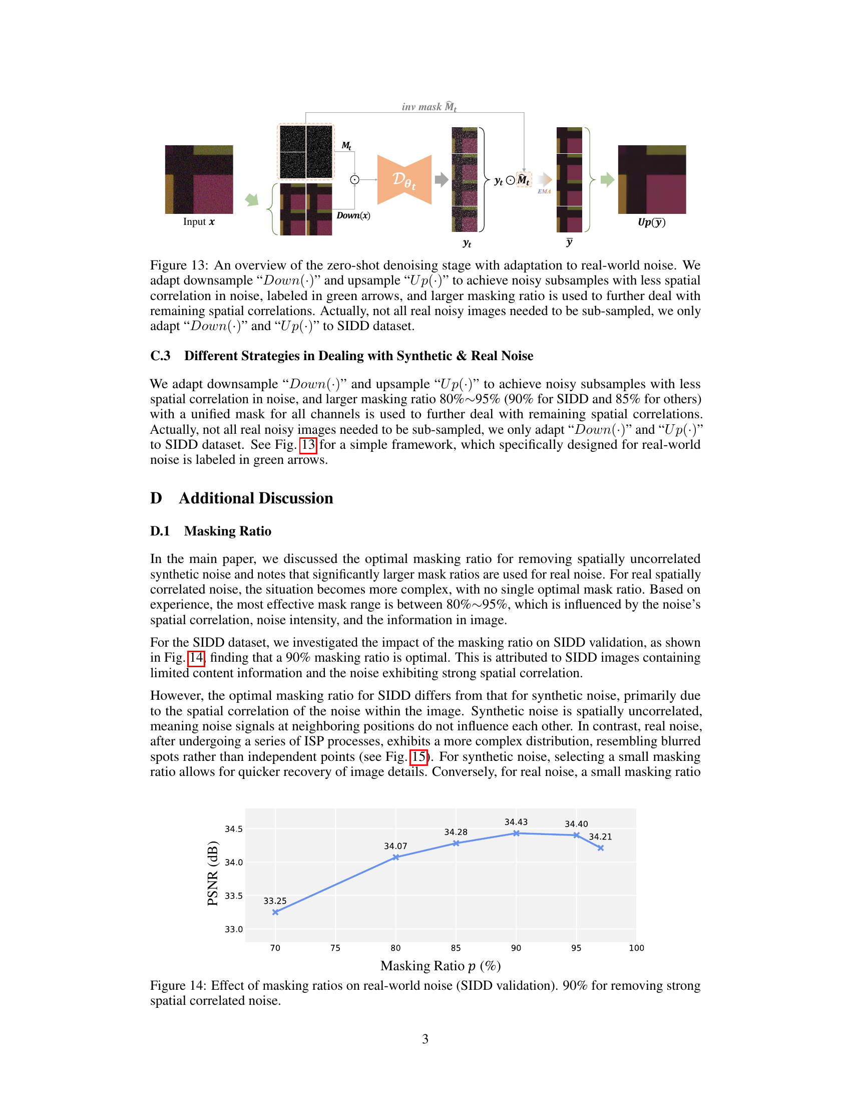
This figure shows the impact of different masking ratios on the denoising performance using synthetic noise. The x-axis represents the masking ratio (percentage of pixels masked), and the y-axis shows the peak signal-to-noise ratio (PSNR) in dB. The plot shows that a masking ratio of around 30% provides the best balance between noise removal and detail preservation. Lower masking ratios result in insufficient noise reduction, while higher ratios lead to over-smoothing and loss of detail. The optimal ratio of 30% is specific to synthetic noise.

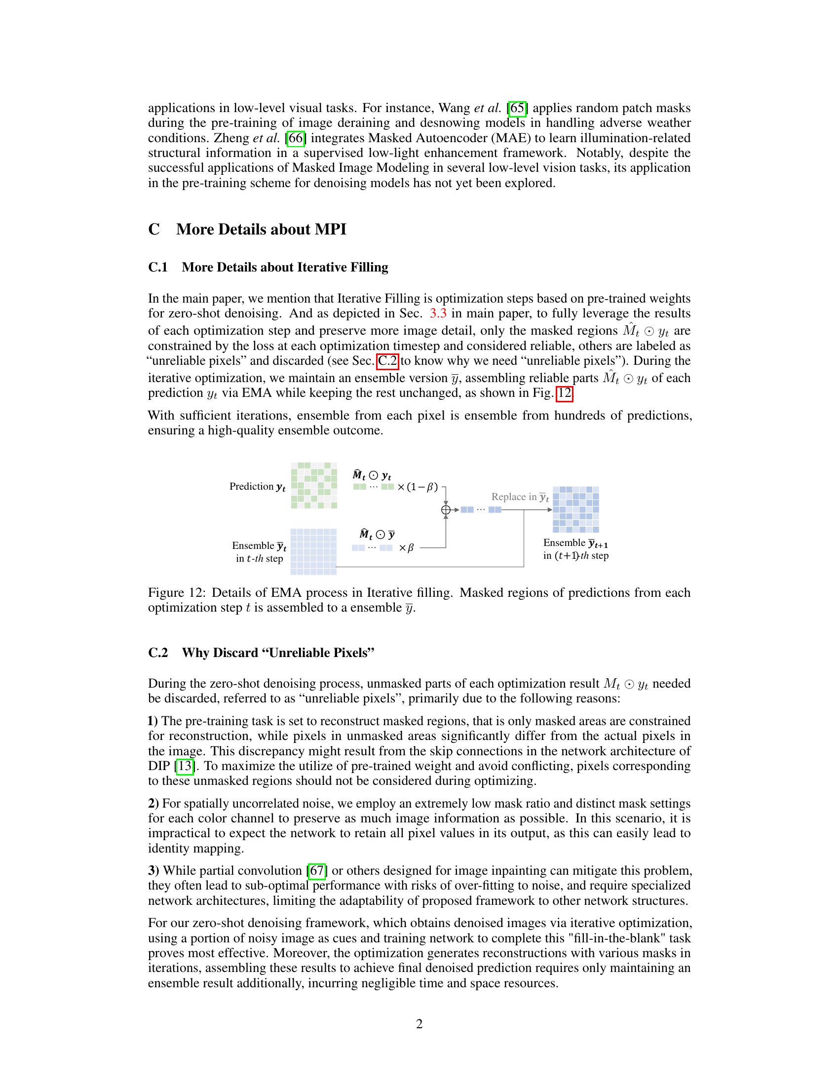
This figure illustrates the Exponential Moving Average (EMA) process used in the Iterative Filling step of the Masked Pre-train then Iterative fill (MPI) method. In each iteration (t), the model generates predictions (yt). Only the predictions for the masked regions (Mt⊙yt) are considered reliable and are used to update the ensemble (ỹt). The contribution of each step’s reliable predictions is weighted by β, an exponential weight. Unreliable pixels are kept unchanged. This process continues across multiple iterations (T) to refine the denoised output.

This figure illustrates the zero-shot denoising process with adaptations for real-world noise. A downsampling step reduces spatial correlations in the noisy image before processing. The model processes the downsampled image using masked pre-training and iterative filling, with the resulting prediction combined using EMA (Exponential Moving Average). Finally, an upsampling step restores the denoised image to its original resolution. The green arrows highlight the downsampling and upsampling operations, which are only applied to the SIDD dataset.

This figure shows the impact of different masking ratios on the performance of the denoising model. The x-axis represents the masking ratio (percentage of pixels masked), while the y-axis represents the PSNR (Peak Signal-to-Noise Ratio), a metric that measures image quality. The plot shows an optimal masking ratio of around 30% for synthetic noise. A lower ratio doesn’t remove enough noise, while a higher ratio leads to over-smoothing, reducing detail. This finding is crucial for balancing noise reduction and detail preservation in the denoising process.
This figure illustrates the two-stage process of the Masked Pre-train then Iterative fill (MPI) method. The first stage, Masked Pre-training, involves training a model (Dθ) to reconstruct natural images from which random patches have been masked. The learned weights (θ) from this stage are then used in the second stage, Iterative Filling. In this stage, the model, initialized with the pre-trained weights, iteratively refines its prediction of a single noisy image (x) by focusing on reconstructing masked portions of the image. The process repeats for ‘T’ steps, ultimately producing a final denoised prediction (y). The inclusion of the pre-trained model improves both speed and quality compared to training a model from scratch for each image.
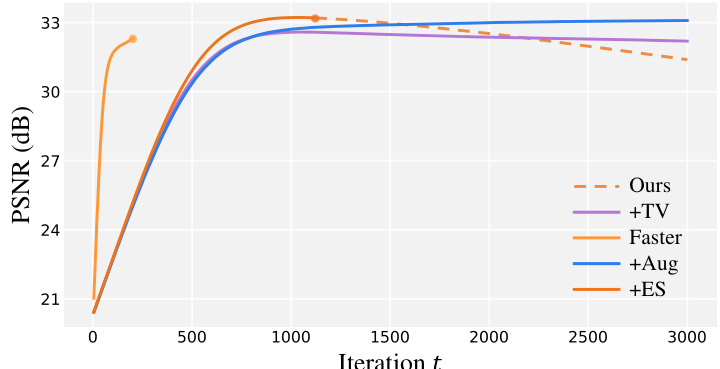
The figure shows the impact of different regularization techniques on the performance of the zero-shot denoising method. Total Variation (TV) regularization, data augmentation, and early stopping are compared to the original method. The results show that early stopping provides the best balance between performance and computational cost.
This figure illustrates the process of adapting the zero-shot denoising method to handle real-world noise. Real-world noise often exhibits strong spatial correlations, which standard masking techniques struggle with. To address this, the model incorporates downsampling and upsampling steps. The downsampling reduces spatial correlation before denoising, and the upsampling restores the image to its original resolution after processing. The figure also highlights the use of a larger masking ratio (80%-95%) to further mitigate the impact of remaining spatial correlations. Notably, this adaptation is specifically applied to the SIDD dataset; not all images undergo downsampling and upsampling.
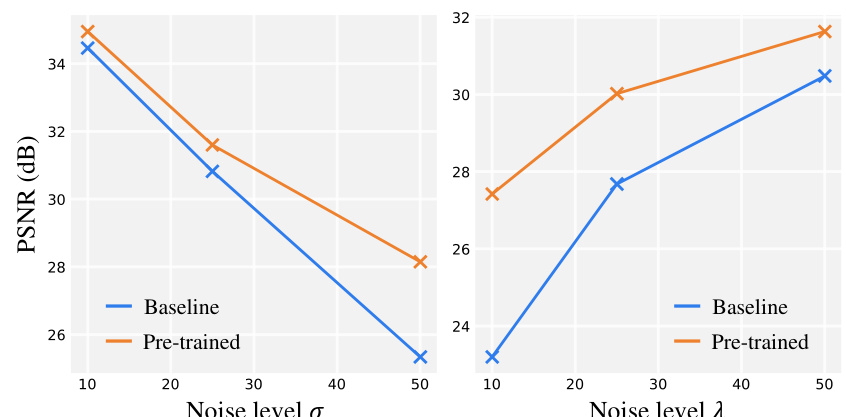
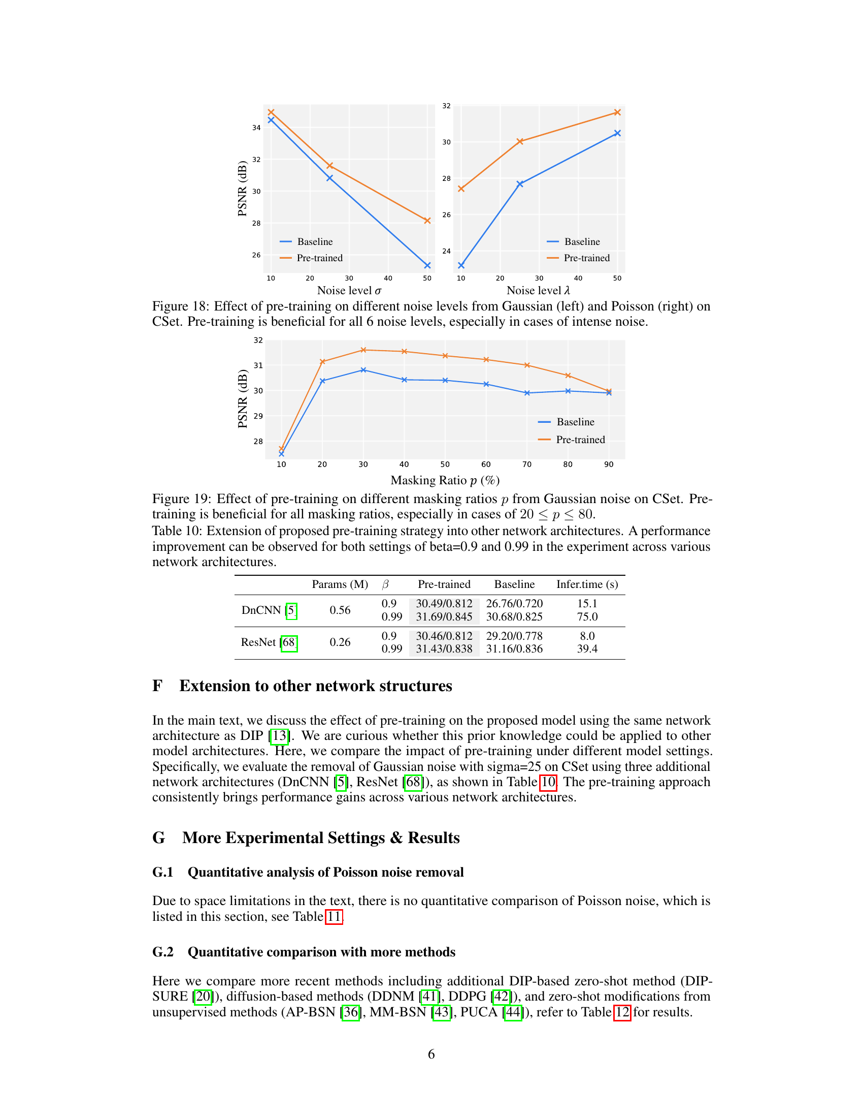
This figure shows the impact of pre-training on the performance of a denoising model at various noise levels. The left panel shows results for Gaussian noise, while the right panel presents results for Poisson noise. Both panels display the PSNR (peak signal-to-noise ratio) against different noise levels (σ for Gaussian and λ for Poisson). Two lines are plotted in each panel, one for the baseline model (trained without pre-training), and one for the model trained using the paper’s proposed masked pre-training approach. The plots illustrate that pre-training significantly improves denoising performance, particularly at higher noise levels, showcasing the effectiveness of the proposed method.

This figure shows the results of an experiment comparing the performance of a denoising model with and without pre-training on different noise levels. The results show that pre-training significantly improves performance on all noise levels, particularly with stronger noise. This is because pre-training provides the model with a better foundation for understanding and removing noise patterns, which helps to reduce overfitting to specific noise characteristics and improve generalization across various noise levels. The left plot shows results for Gaussian noise, while the right plot shows results for Poisson noise.

This figure shows a visual comparison of the denoising results from various methods on a specific noisy image patch (SIDDval_34_22) from the SIDD validation dataset. It allows for a qualitative assessment of the performance of each method in terms of noise reduction and detail preservation. The methods compared include the proposed ‘Ours’ method, along with several baselines and state-of-the-art zero-shot and other denoising techniques, such as DIP-SURE, DDNM, DDPG, MM-BSN and PUCA. The Ground Truth (GT) is also provided for reference.

This figure demonstrates the effectiveness of the proposed MPI method for image denoising. Subfigure (a) compares the computational cost and performance of MPI against other zero-shot denoising methods, highlighting its speed advantage. Subfigure (b) showcases MPI’s superior generalization ability across various noise types compared to both zero-shot and supervised/unsupervised approaches. Finally, subfigure (c) illustrates MPI’s capability to effectively denoise real-world images with spatial noise correlation, using images from the SIDD and FMD benchmark datasets.

This figure provides a visual overview of the Masked Pre-train then Iterative fill (MPI) paradigm. It shows the two main stages: 1) Masked Pre-training, where a model learns to reconstruct masked natural images, and 2) Iterative filling, which uses the pre-trained weights to iteratively refine a noisy image. The iterative process involves masking parts of the image, making predictions, and updating the model weights to better reconstruct the masked regions. This process is repeated multiple times, leading to improved denoising. The figure highlights how the pre-trained knowledge enables faster and better zero-shot denoising compared to traditional methods.
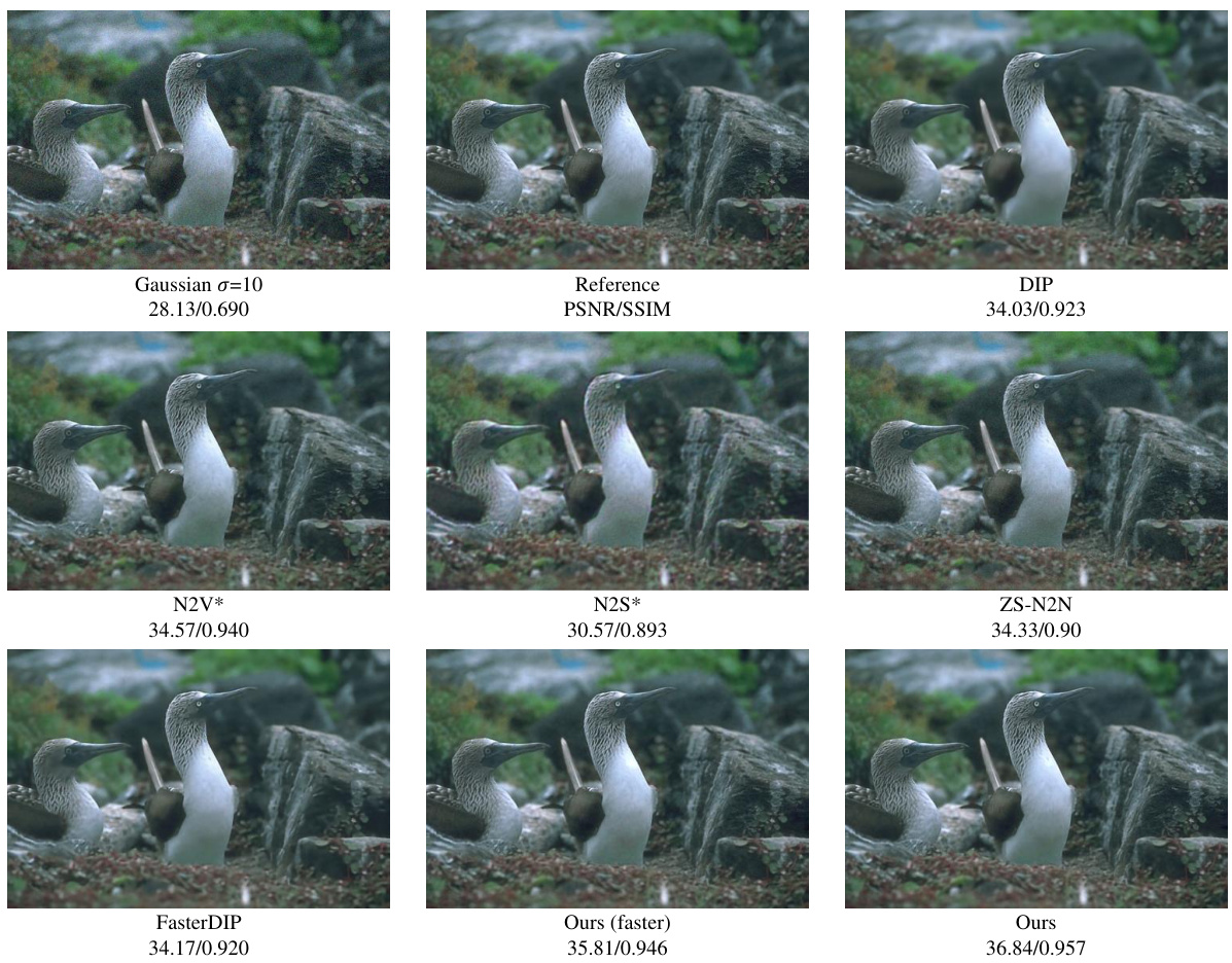
This figure compares the denoising performance of various methods on a noisy patch from the CBSD dataset using Gaussian noise with a standard deviation of 10. The methods compared include DIP, N2V*, N2S*, ZS-N2N, FasterDIP, and the proposed method (Ours). The reference image is provided for comparison. The results are presented in terms of PSNR and SSIM values, which are quantitative metrics of image quality.

This figure demonstrates the superiority of the proposed method (Ours) compared to existing zero-shot and supervised/unsupervised image denoising methods across three key aspects: computational cost, generalization ability, and real-world noise removal. (a) shows the reduced inference time of the proposed method. (b) highlights the improved generalization across different noise types. (c) showcases the effectiveness on real-world noisy images from SIDD and FMD benchmark datasets.
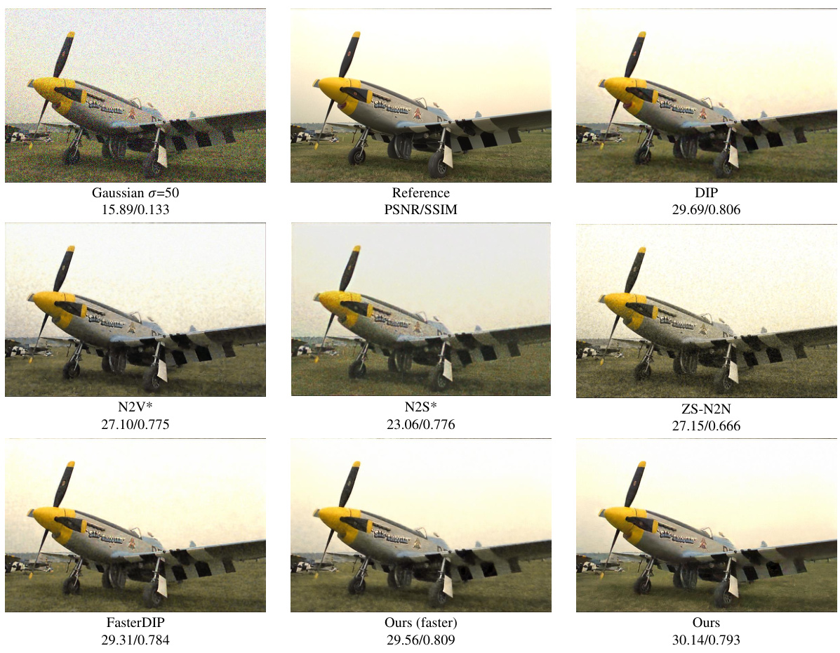
This figure shows the qualitative and quantitative results of the proposed MPI method on Gaussian and Poisson noise. The results are compared against several state-of-the-art denoising methods. The qualitative comparison shows the visual results of denoising on noisy patches from the CBSD-44 and McMaster-14 datasets. The quantitative comparison shows the PSNR and SSIM values for each method.

This figure shows a qualitative comparison of different image denoising methods on a noisy patch from the CBSD dataset with Poisson noise (λ=10). The comparison includes the original noisy image, the ground truth (reference) image, and results from DIP, N2V*, N2S*, ZS-N2N, FasterDIP, the faster version of the proposed MPI method, and the proposed MPI method. The visual results demonstrate the relative performance of each method in terms of noise reduction and detail preservation.

This figure compares the denoising results of different methods on a CBSD dataset patch with Poisson noise (λ=25). The methods compared include DIP, N2V*, N2S*, ZS-N2N, FasterDIP, the proposed ‘Ours (faster)’ method, and the full ‘Ours’ method. The figure visually demonstrates the performance differences of each method in terms of noise reduction and detail preservation.

The figure shows a qualitative comparison of denoising results on a noisy patch from the CBSD dataset with Poisson noise (λ=50). It compares the performance of different methods including DIP, N2V*, N2S*, ZS-N2N, FasterDIP, and the proposed method (MPI). The results demonstrate the superior performance of the MPI method in terms of noise removal and detail preservation compared to the other methods.

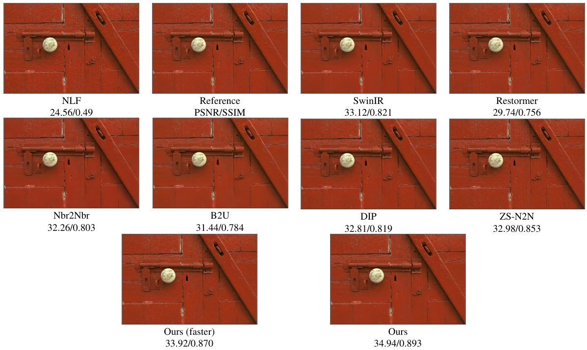
This figure compares the results of different denoising methods on a noisy patch from the Kodak dataset, where the noise is Salt and Pepper noise with density d=0.045. The methods compared include SwinIR, Restormer, Neighbor2Neighbor, Blind2Unblind, DIP, ZS-N2N, and the proposed MPI method (both faster and full versions). The figure shows the visual quality of the denoised images produced by each method, highlighting the performance differences.
This figure compares the feature distributions obtained from a model with and without pre-training using Kernel Canonical Correlation Analysis (CKA) and Principal Component Analysis (PCA). The results show that pre-trained weights significantly impact the feature distributions and improve the performance in image restoration. The pre-trained model focuses on restoring the complete image, while the untrained model focuses only on the masked areas.
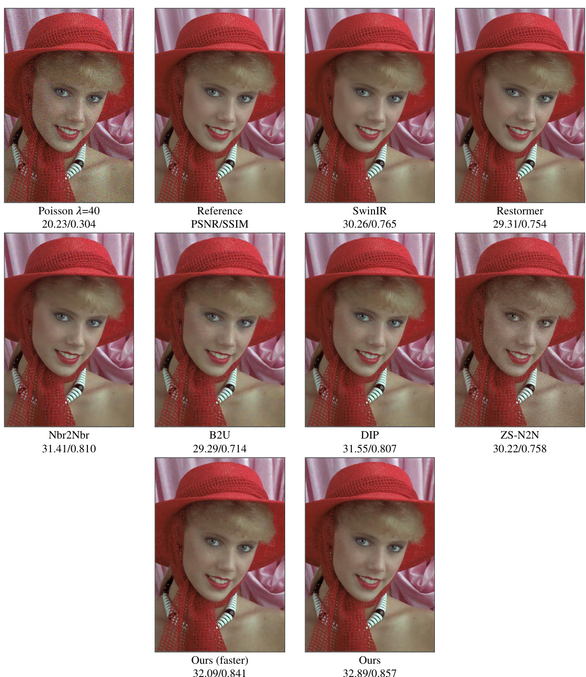
This figure compares the denoising performance of different methods on a noisy patch from the Kodak dataset with Poisson noise (λ=40). The comparison includes several supervised and unsupervised methods, along with the proposed MPI method. The results show that MPI achieves superior denoising quality and better detail preservation compared to the other methods. This demonstrates the generalization capability of the proposed method to various unseen noise types.

This figure shows a qualitative comparison of denoising results on a real-world noisy image patch from the PolyU dataset. The comparison includes the noisy image, the ground truth, and denoising results from several methods (DIP, N2V*, N2S*, ZS-N2N, FasterDIP, MPI (faster version), and MPI). The goal is to visually demonstrate the performance of MPI in removing real-world noise while preserving image details. Each method’s PSNR and SSIM scores are also displayed.

This figure shows the qualitative comparison of denoising results on real noisy images from SIDD and PolyU datasets. The results demonstrate the effectiveness of the proposed method (Ours) in removing real-world noise compared to other existing methods (DIP, N2V*, N2S*, ZS-N2N, FasterDIP). It highlights the method’s ability to preserve image details while effectively removing noise.
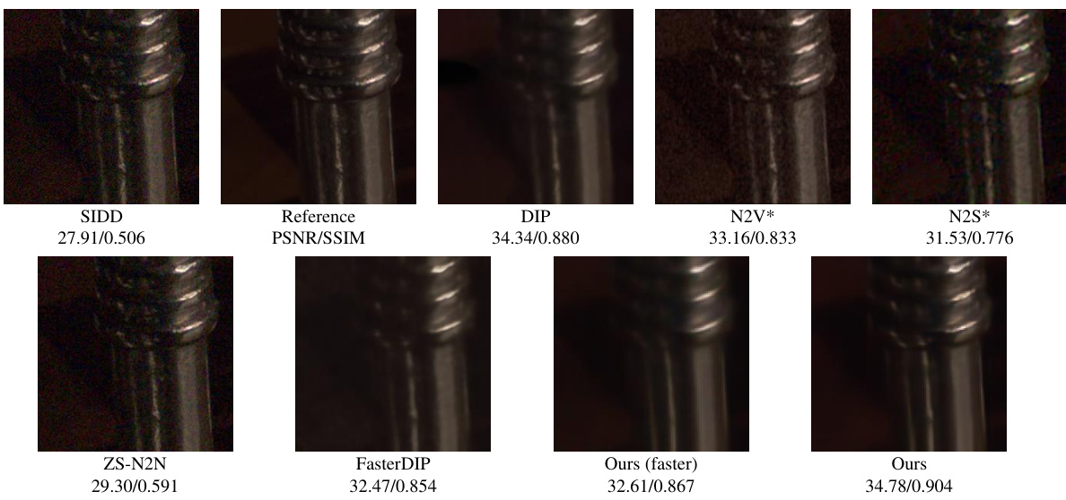
This figure shows a qualitative comparison of denoising results on a real noisy image patch from the SIDD dataset. The comparison includes the noisy image, the ground truth (reference), and the denoised images generated by various methods including DIP, N2V*, N2S*, ZS-N2N, FasterDIP, and the proposed method (MPI). The results illustrate the effectiveness of the authors’ proposed method in achieving high quality results with preserved details compared to the other methods.

This figure shows a qualitative comparison of different denoising methods on a specific noisy patch from the SIDD validation dataset (SIDDval_34_22). It visually compares the results of DIP, N2V*, N2S*, ZS-N2N, FasterDIP, and the proposed ‘Ours (faster)’ and ‘Ours’ methods against the ground truth image. The comparison allows a visual assessment of the relative performance of each method in terms of noise reduction and detail preservation.
More on tables

This table presents a quantitative comparison of the generalization performance of various image denoising methods on the Kodak dataset. The methods were initially trained using Gaussian noise with a standard deviation of 25. The table evaluates their performance across five different unseen noise types: Gaussian noise with varying standard deviations, Poisson noise with varying lambda values, Noise Level Function (NLF) noise, speckle noise with varying variance values, and salt-and-pepper noise with varying density values. The average PSNR and SSIM values across these different noise types are reported for each method, providing an assessment of their ability to generalize to unseen noise conditions. The results indicate that the proposed method shows superior generalization capabilities compared to others.

This table presents a quantitative comparison of different image denoising methods on three real-world noisy image datasets: SIDD, PolyU, and FMD. The comparison is based on Peak Signal-to-Noise Ratio (PSNR) and Structural Similarity Index (SSIM) metrics, which measure the quality of the denoised images. The table also includes the average inference time for each method, highlighting the computational efficiency of the proposed MPI method. The results demonstrate the superior performance of the MPI method, particularly its faster inference speed, compared to existing methods.

This table presents the ablation study results on the impact of pre-trained weights on the performance of the proposed zero-shot denoising method. It compares the performance of the model with and without pre-training on three different datasets: CSet, SIDD, and FMD. The results are presented in terms of PSNR and SSIM values. The table also shows the effect of different values of the exponential weight parameter β on the model’s performance.
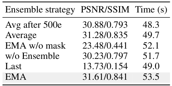
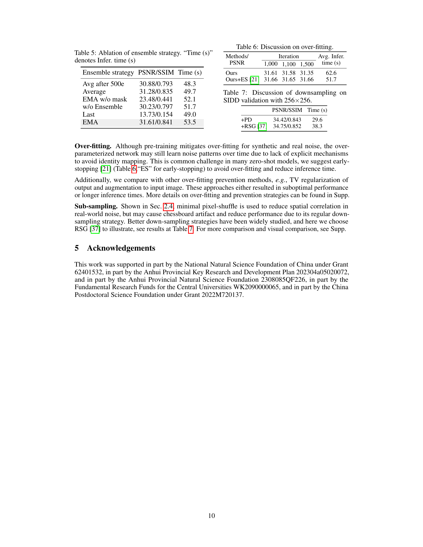
This ablation study analyzes different ensemble strategies for the proposed zero-shot denoising method. The table compares the performance (PSNR/SSIM) and inference time for six different strategies: ‘Avg after 500e’, ‘Average’, ‘EMA w/o mask’, ‘w/o Ensemble’, ‘Last’, and ‘EMA’. The results highlight the impact of the ensemble method on the overall denoising quality and efficiency.

This table presents a quantitative comparison of different image denoising methods on three benchmark datasets (CSet, McMaster, and CBSD) using Gaussian noise with different standard deviations (σ). The results are shown in terms of Peak Signal-to-Noise Ratio (PSNR) and Structural Similarity Index (SSIM). The best results for each metric and dataset are highlighted, and the second-best results are underlined. The supplementary material includes results for Poisson noise removal.

This table shows the results of experiments conducted to evaluate the performance of the proposed pre-training strategy when applied to different network architectures. The table compares the PSNR values obtained using the proposed method with two different values of beta (0.9 and 0.99) across multiple iterations (800, 900, and 1200). The average inference time for each setting is also provided. The purpose is to demonstrate the generalizability and effectiveness of the proposed method across various network architectures.

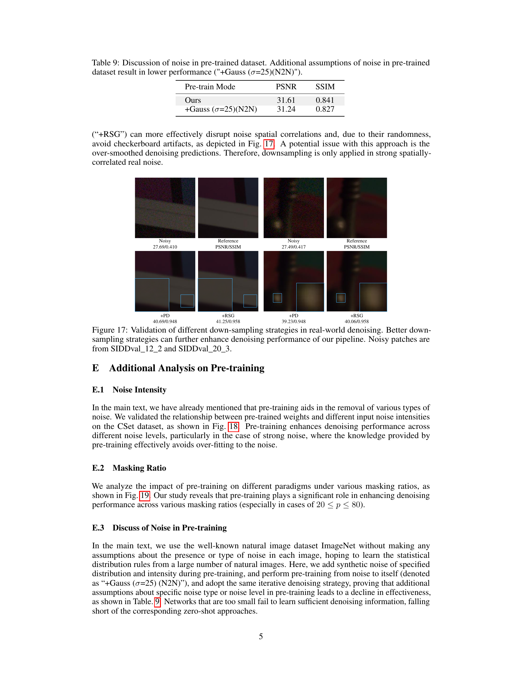
This table compares the performance of the proposed method with and without adding Gaussian noise (σ=25) during pre-training. The results show that adding additional assumptions about the noise during pre-training leads to a decline in effectiveness, indicating the benefit of learning from the natural distribution of images without making additional assumptions about the noise.

This table shows the performance of the proposed Masked Pre-train then Iterative fill (MPI) method on different network architectures (DnCNN and ResNet). It demonstrates that the pre-training approach consistently improves performance across various network architectures, regardless of the beta value used (0.9 or 0.99). The results are presented in terms of PSNR and SSIM, and the average inference time is also shown.

This table presents a quantitative comparison of different image denoising methods on three benchmark datasets (CSet, McMaster, and CBSD) using Gaussian noise with different noise levels (σ = 10, 25, 50). The methods compared include DIP, N2V*, N2S*, ZS-N2N, FasterDIP, and the proposed method (Ours and Ours (faster)). The results are reported in terms of Peak Signal-to-Noise Ratio (PSNR) and Structural Similarity Index (SSIM). The best performing method for each noise level and dataset is highlighted, and the second-best performing method is underlined. Results for Poisson noise removal are available in the supplementary material.

This table presents a quantitative comparison of different image denoising methods on three benchmark datasets (CSet, McMaster, and CBSD) for Gaussian noise removal. The comparison is based on Peak Signal-to-Noise Ratio (PSNR) and Structural Similarity Index (SSIM) metrics, which measure the quality of the denoised images. The table shows the performance of various methods at different levels of Gaussian noise (σ=10, 25, 50). The best results for each noise level and dataset are highlighted, with the second-best results underlined. Additional results for Poisson noise removal are available in the supplementary material.

This table presents a quantitative comparison of different image denoising methods on three datasets (CSet, McMaster, and CBSD) using Gaussian noise with different noise levels (σ = 10, 25, 50). The methods compared include DIP, N2V*, N2S*, ZS-N2N, FasterDIP, and the proposed method (Ours and Ours (faster)). For each method and dataset, the Peak Signal-to-Noise Ratio (PSNR) and Structural Similarity Index (SSIM) are reported. The best results for each noise level are highlighted, and the second-best results are underlined. Additional results for Poisson noise removal are available in the supplementary material.

This table presents a quantitative comparison of the generalization performance of ensemble versions of N2V* and N2S* on the Kodak dataset. It evaluates the performance of these methods across five different noise types: Gaussian (σ=25), Gaussian (σ∈[10,50]), Poisson (λ∈[10,50]), NLF, Speckle (v∈[10,50]), and S&P (d∈[0.02,0.05]). The results show the average PSNR and SSIM scores achieved by each method for each noise type, providing insights into their generalization capabilities across various noise conditions.

This table presents a quantitative comparison of different image denoising methods on three real-world noisy image datasets: SIDD, PolyU, and FMD. The metrics used for comparison are PSNR and SSIM, common measures of image quality after denoising. The table also includes the average inference time for each method, showing the computational efficiency.

This table presents a quantitative comparison of different image denoising methods on three datasets (CSet, McMaster, and CBSD) using Gaussian noise with standard deviations of 10, 25, and 50. The methods compared include DIP, N2V*, N2S*, ZS-N2N, FasterDIP, and the proposed method (Ours and Ours (faster)). The results are reported in terms of PSNR and SSIM, showing the superior performance of the proposed method in most scenarios. The ‘Supp.’ reference likely indicates additional results are available in a supplementary document. The table also includes average inference times, highlighting the speed advantage of the proposed method.
Full paper#
