↗ OpenReview ↗ NeurIPS Homepage ↗ Chat
TL;DR#
Simple bilevel optimization (SBO) problems, minimizing an upper-level objective over the optimal solution set of a convex lower-level objective, pose significant challenges. Existing methods often suffer from slow convergence or strong assumptions. This paper addresses these challenges by proposing a penalization framework that connects approximate solutions of the original SBO problem and its reformulated counterparts. This allows for flexibility in handling various smoothness and convexity assumptions, using different algorithms with distinct convergence results.
The paper introduces a penalty-based Accelerated Proximal Gradient (APG) algorithm. Under an a-Hölderian error bound and mild assumptions, this algorithm achieves an (ε, εβ)-optimal solution. The results improve further when strong convexity is present. The framework is extended to general nonsmooth functions, showcasing its versatility and effectiveness. Numerical experiments validate the effectiveness of the algorithms, highlighting their superior performance compared to existing methods.
Key Takeaways#
Why does it matter?#
This paper is crucial for researchers in bilevel optimization due to its novel penalization framework that provides non-asymptotic convergence rates for simple bilevel problems, addressing limitations of existing methods. It offers flexible algorithms adaptable to various assumptions on problem structures and provides valuable complexity results, opening avenues for future work in handling nonsmooth and nonconvex cases. Its adaptable methods enhance the applicability and efficiency of SBO across diverse applications.
Visual Insights#

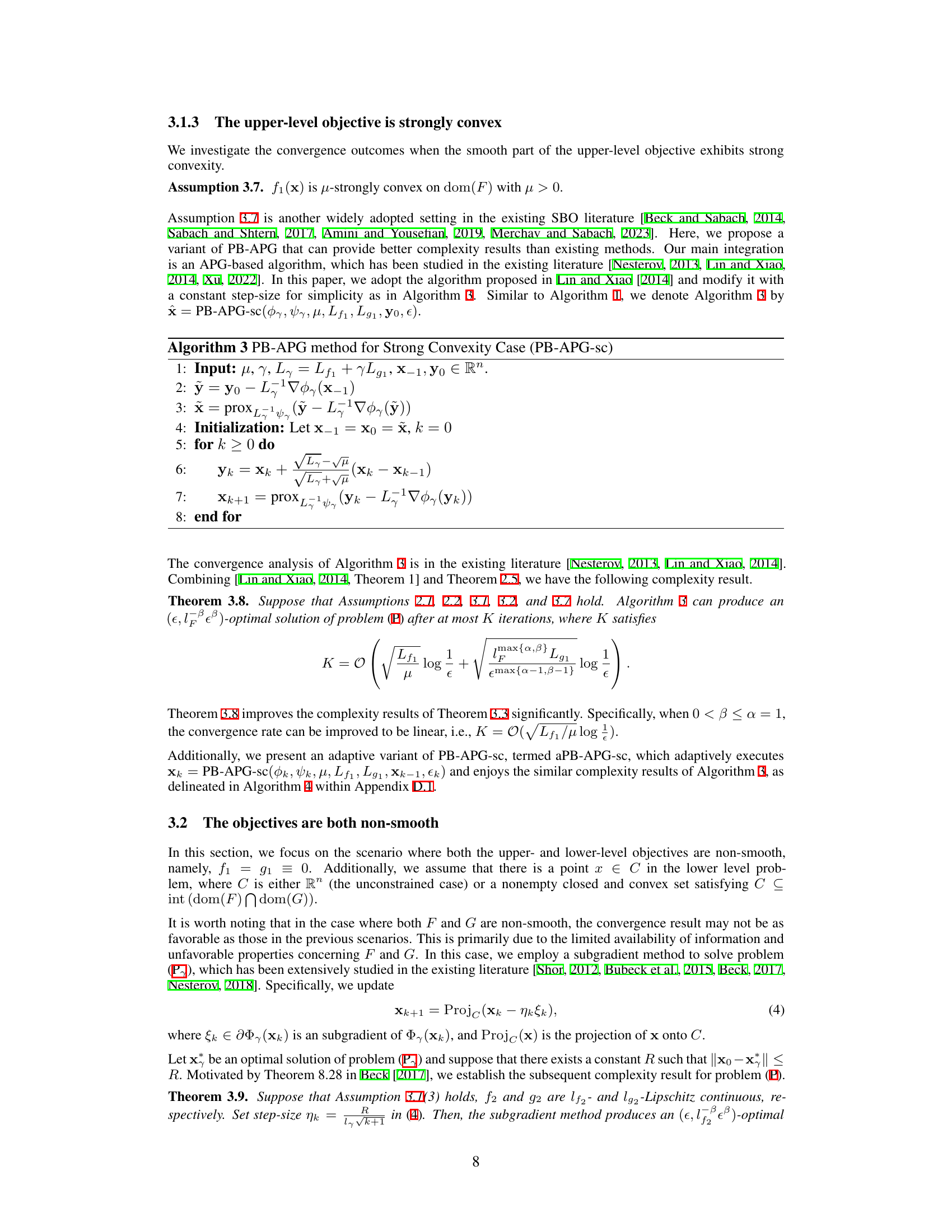
This figure presents a comparison of different optimization methods’ performance on a Logistic Regression Problem (LRP). It shows the convergence of the residuals of the lower-level objective (G(x) - G*) and the upper-level objective (F(x) - F*) over time (in seconds). The plot helps to visualize the speed and efficiency of various algorithms in solving this bilevel optimization problem. Different line styles and colors represent different algorithms.

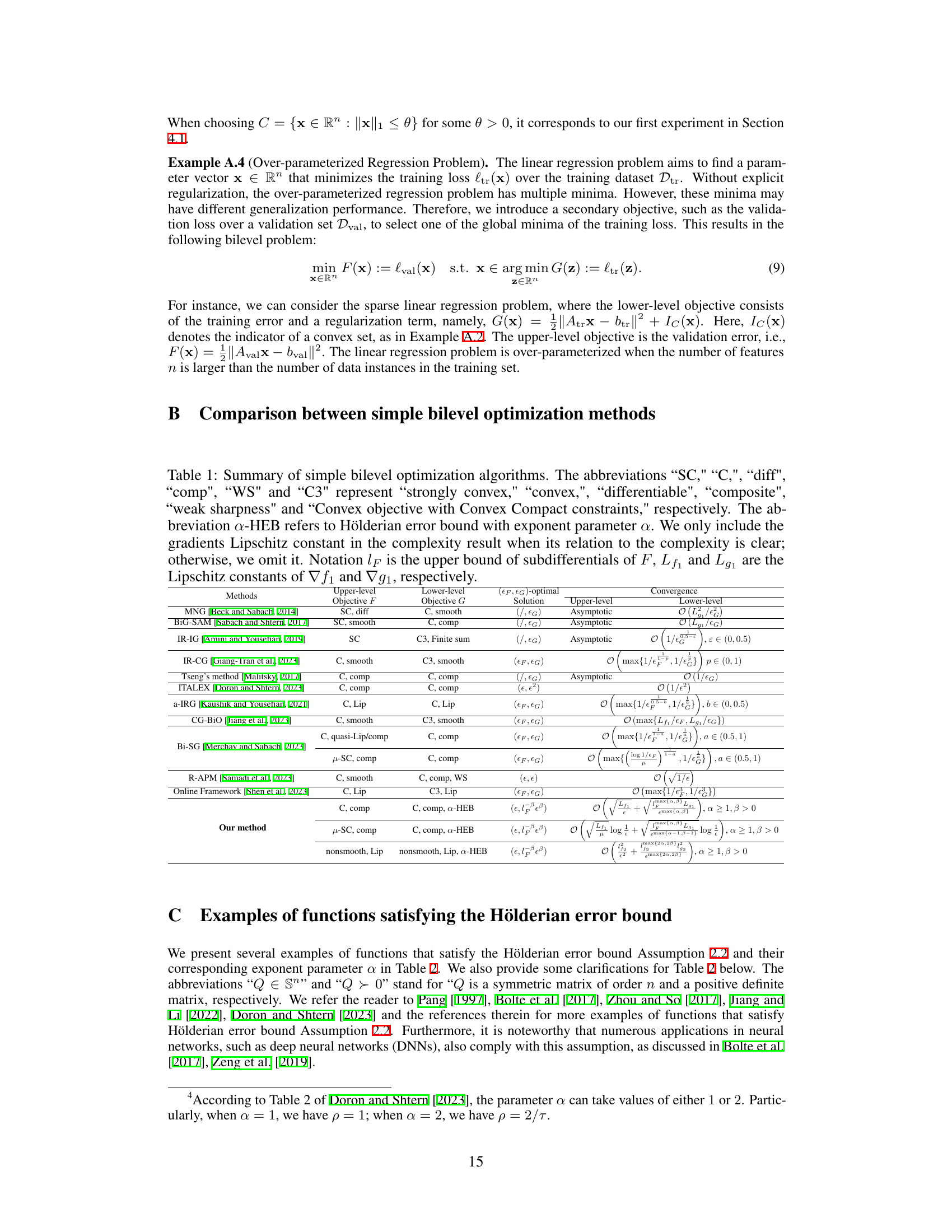
This table summarizes several existing simple bilevel optimization algorithms. For each algorithm, it lists the assumptions on the objective functions (strong convexity, smoothness, convexity, etc.), the type of solution obtained, and the corresponding convergence rate. It also indicates whether or not the algorithm’s complexity depends on specific Lipschitz constants.
In-depth insights#
Hölderian Error Bounds#
Hölderian error bounds, in the context of optimization, quantify the rate at which a function’s value approaches its minimum as the distance to the optimal solution set decreases. Crucially, they provide a quantitative measure of the problem’s conditioning, indicating how well-behaved the optimization landscape is. A strong Hölderian error bound, with a large exponent α, implies fast convergence, suggesting that algorithms should find solutions efficiently. Conversely, a weak bound (small α) signals potential difficulties, such as slow convergence or sensitivity to initialization. The parameter p scales the bound, and while not as impactful as α, it affects the overall convergence rate. The paper’s utilization of Hölderian error bounds allows for nuanced complexity analysis, providing a theoretical basis for the proposed algorithms’ performance and demonstrating that the developed methods can find approximate solutions within specific iteration bounds, even in the presence of non-smooth functions.
Penalty Framework#
The Penalty Framework section is crucial as it bridges the theoretical gap between the original simple bilevel optimization problem (P) and its penalized reformulation (Pγ). It rigorously establishes the relationship between approximate solutions of both problems, showing that solving the penalized problem (Pγ) approximately yields an approximate solution for (P). This is achieved through the use of Hölderian error bounds, which characterize the relationship between approximate solutions and the optimal solution set. This framework is significant because it allows for the application of various optimization algorithms (e.g., APG) to the simpler unconstrained penalized problem (Pγ), providing a direct pathway to approximate solutions of the complex bilevel problem (P). The framework’s adaptability to varying assumptions regarding smoothness and convexity enhances its versatility and effectiveness across a broader range of problems. Finally, the theorems derived within this framework provide non-asymptotic complexity bounds, offering concrete estimates of the algorithm’s efficiency. This detailed analysis underscores the penalty framework’s pivotal role in translating theoretical guarantees into practical algorithms for solving simple bilevel optimization problems.
APG Algorithm#
The APG (Accelerated Proximal Gradient) algorithm is a powerful optimization technique particularly well-suited for solving problems involving composite objective functions, which are sums of smooth and nonsmooth components. Its core strength lies in its ability to achieve accelerated convergence rates compared to standard gradient methods. In the context of bilevel optimization, where an upper-level objective depends on the solution of a lower-level problem, APG’s efficiency is particularly valuable because bilevel problems are often computationally challenging. The paper leverages APG’s efficiency by incorporating it within a penalty-based framework to solve simple bilevel optimization problems, demonstrating its applicability and efficacy in a complex setting. The adaptive versions of APG, incorporating warm-start mechanisms and dynamically adjusting penalty parameters, further enhance its practical performance offering robustness and potentially superior convergence characteristics in real-world applications where parameter tuning is difficult.
Adaptive PB-APG#
The adaptive penalty-based accelerated proximal gradient (aPB-APG) method presents a significant advancement in bilevel optimization by dynamically adjusting the penalty parameter and solution accuracy. Unlike traditional methods requiring predefined penalty parameters, which can be challenging to determine, aPB-APG leverages an iterative process, refining the penalty parameter at each iteration. This adaptive approach enhances the algorithm’s efficiency and robustness. The method’s effectiveness is further boosted by incorporating a warm-start mechanism, utilizing the previous iteration’s solution as the starting point for the next. This not only accelerates convergence but also enhances the overall performance. Theoretical analysis supports the algorithm’s effectiveness and provides complexity results, demonstrating the algorithm’s convergence properties under various conditions. The aPB-APG method is shown to be particularly effective when dealing with problems involving composite functions where the upper level objectives are strongly convex, demonstrating superior performance compared to existing approaches.
Future Works#
The authors could explore extending their penalty-based framework to tackle more complex bilevel optimization problems, such as those with non-convex upper-level objectives or non-convex lower-level objectives. Investigating the impact of different penalty functions and their parameters on convergence speed and solution quality is crucial. Another avenue for future work involves developing more efficient algorithms for solving the penalized single-level problem, especially for large-scale problems. A direct comparison to other state-of-the-art bilevel optimization methods on a wider range of benchmark datasets would strengthen the paper’s claims. Moreover, exploring the theoretical guarantees under weaker assumptions, such as relaxing the Hölderian error bound condition or the strong convexity assumption, could broaden the applicability of their framework. Analyzing the sensitivity of the algorithm to parameter choices and developing adaptive or robust versions would make the methods more practical. Finally, the application of this framework to real-world machine learning problems, such as hyperparameter optimization and meta-learning, deserves in-depth investigation to confirm the empirical effectiveness.
More visual insights#
More on figures

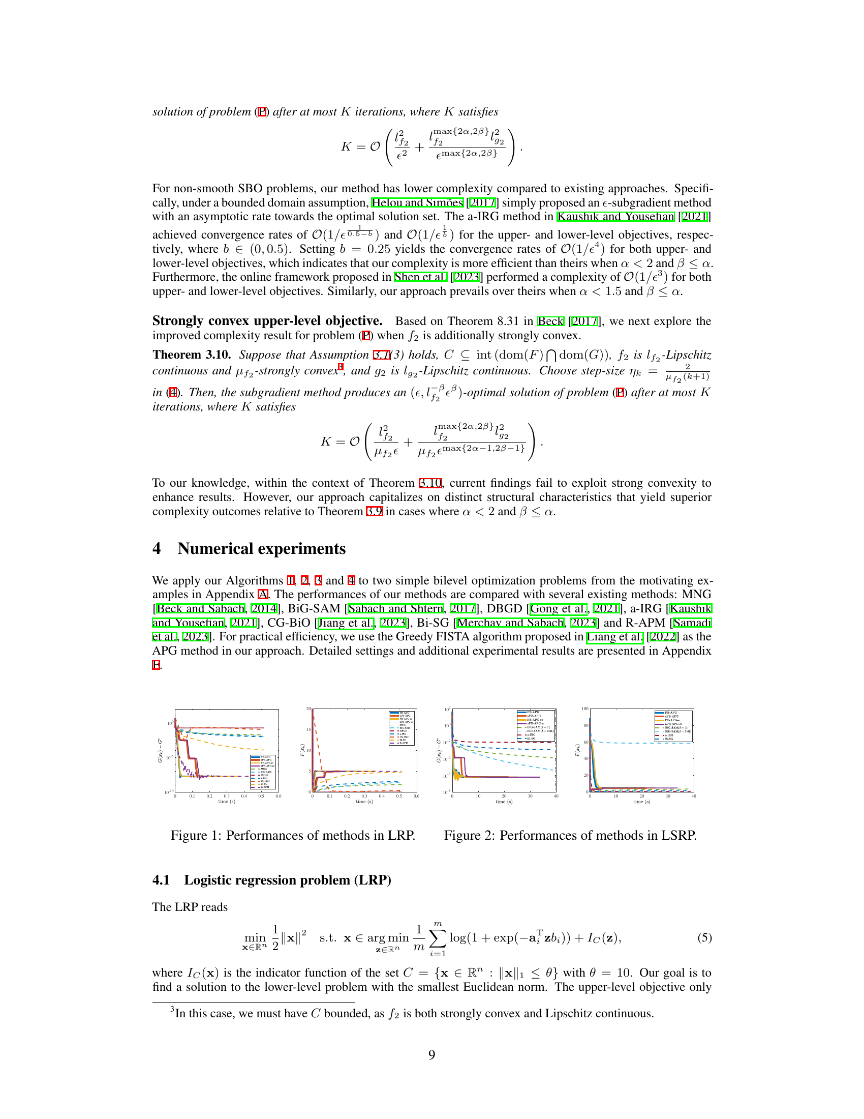
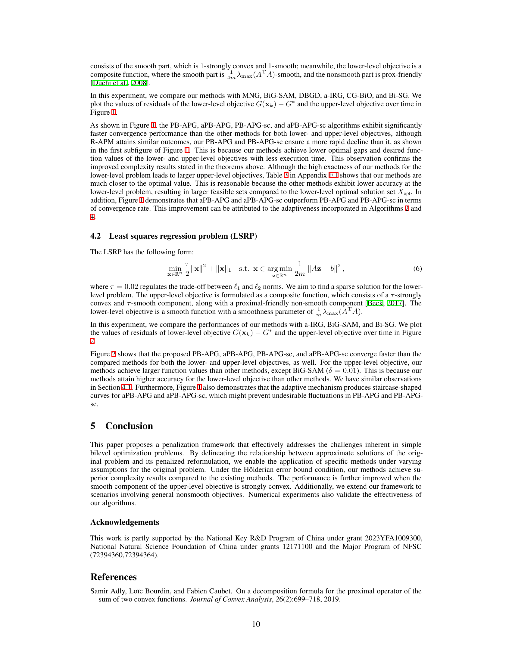
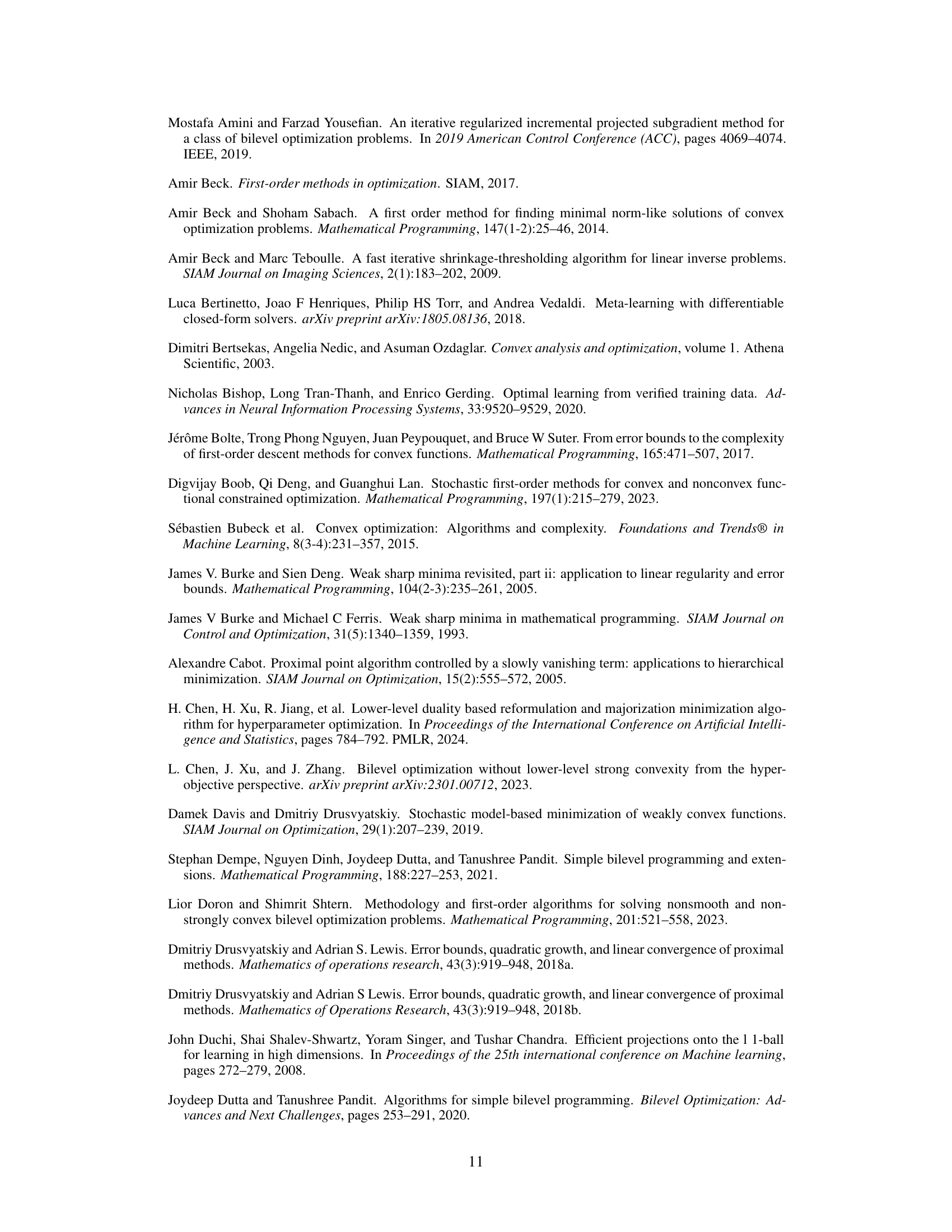
This figure shows the performance comparison of different optimization methods (PB-APG, aPB-APG, PB-APG-sc, aPB-APG-sc, MNG, BIG-SAM, DBGD, a-IRG, CG-BiO, Bi-SG, and R-APM) on the Logistic Regression Problem (LRP). The plots illustrate the convergence of the lower-level objective (G(x)-G*) and the upper-level objective (F(x)) over time. It demonstrates the faster convergence of the proposed penalty-based methods (PB-APG, etc.) compared to the existing methods.

This figure compares the performance of several bilevel optimization methods on the Logistic Regression Problem (LRP). The x-axis represents time (in seconds), and the y-axis shows the values of the residuals for both the lower-level objective (G(xk) - G*) and the upper-level objective (F(xk) - F*). The figure demonstrates that the proposed PB-APG, aPB-APG, PB-APG-sc, and aPB-APG-sc algorithms exhibit significantly faster convergence than other methods for both lower- and upper-level objectives, although R-APM attains similar outcomes for the lower level objective.

The figure shows the performance comparison of different optimization methods on the Logistic Regression Problem (LRP). The x-axis represents the time in seconds, and the y-axis shows the residuals of the lower-level objective (G(xk) - G*) and the upper-level objective (F(xk) - F*). The plot demonstrates that PB-APG, aPB-APG, PB-APG-sc, and aPB-APG-sc algorithms converge significantly faster than other methods for both lower- and upper-level objectives.

This figure compares the performance of various optimization methods on the Logistic Regression Problem (LRP). The x-axis represents time, and the y-axis shows the residuals (difference between the current value and optimal value) for both the lower-level objective (G(x)-G*) and the upper-level objective (F(x)-F*). The plot showcases the convergence speed and accuracy of each method in reaching the optimal solution, allowing for a visual comparison of their efficiency and effectiveness.
More on tables

This table summarizes various simple bilevel optimization algorithms, comparing their convergence properties and assumptions. It shows the type of objective functions (strongly convex, convex, differentiable, composite), the type of solution achieved ((εF, εG)-optimal, asymptotic), and the computational complexity. It also notes the assumptions used by each method, such as weak sharpness or Hölderian error bound.

This table summarizes several existing simple bilevel optimization algorithms, highlighting their assumptions (convexity, smoothness, strong convexity, weak sharpness), the type of optimal solution they achieve, and their convergence rates. It serves as a comparison to the proposed algorithms in the paper.
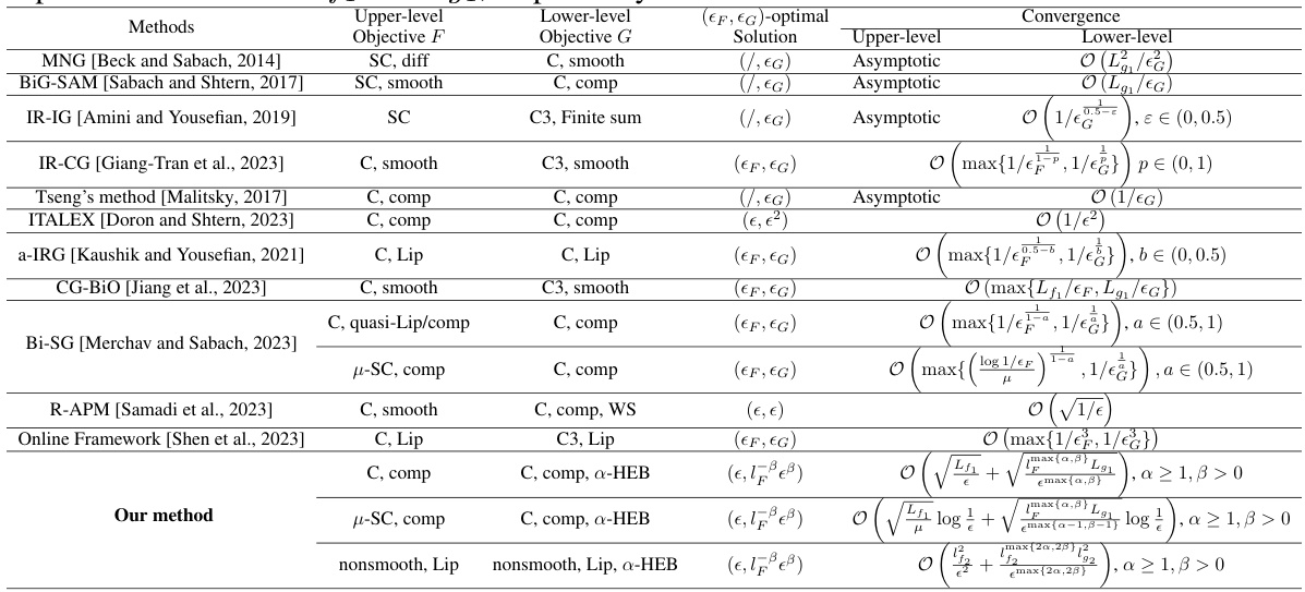
This table summarizes various simple bilevel optimization algorithms, comparing their assumptions (convexity, smoothness, etc.), the type of solution they guarantee, and their convergence rates. It highlights the differences in assumptions and performance between existing methods and sets the stage for the proposed algorithms in the paper.

This table compares various simple bilevel optimization algorithms in terms of their convergence properties, assumptions on the objective functions, and the type of optimal solution obtained. It highlights differences in the assumptions made about convexity, smoothness, and strong convexity of the objective functions, and the complexity of achieving an (εF, εG)-optimal solution. The table helps illustrate the trade-offs involved in choosing a particular algorithm for a given problem based on desired properties and computational resources.

This table compares several simple bilevel optimization algorithms, highlighting their assumptions, convergence results, and optimal solutions. It summarizes key aspects such as the convexity and smoothness of the objective functions (upper and lower levels), and the type of optimal solution achieved. The table also shows the convergence rates achieved by each method, which are often expressed in terms of the error tolerance (ε) and other parameters.

This table summarizes the key characteristics and convergence results of various simple bilevel optimization algorithms. It compares their assumptions (convexity, smoothness, strong convexity, etc.), the type of solution they guarantee (ε, ε)-optimal, asymptotic convergence, etc.), and their complexity bounds. The table is useful for understanding the relative strengths and weaknesses of different approaches to solving simple bilevel optimization problems and placing the proposed methods in the context of existing literature.

This table summarizes several existing simple bilevel optimization methods, comparing their assumptions (convexity, smoothness, etc.), the type of solution they guarantee, and their convergence rates. It highlights the differences in assumptions and performance across various algorithms, setting the stage for the proposed approach.

This table compares several simple bilevel optimization methods, highlighting their assumptions (convexity, smoothness, etc.), the type of solution they find (e.g., (εF, εG)-optimal), and their convergence rates. It provides a concise overview to contrast the proposed method with existing approaches in the literature.

This table compares various simple bilevel optimization algorithms in terms of their assumptions (convexity, smoothness, etc.), the type of optimal solution they find, and their convergence rates. It helps to understand the context of the proposed algorithms in the paper and shows how they improve on existing methods.

This table summarizes several simple bilevel optimization algorithms, comparing their assumptions, convergence rates, and optimality guarantees for both upper- and lower-level objectives. It highlights the differences in the assumptions made (strong convexity, smoothness, composite structure), the type of optimality achieved (asymptotic, (ε,ε)-optimal), and the complexity bounds (in terms of the number of iterations or oracle calls).
Full paper#
