TL;DR#
Linear Programming (LP) is a fundamental optimization problem with broad applications. Recently, Graph Neural Networks (GNNs) have shown promise in solving LPs, but theoretical understanding lagged behind empirical results. Existing theories required large GNNs for accurate solutions, contradicting observed efficiency of smaller networks. This created a critical gap between theory and practice.
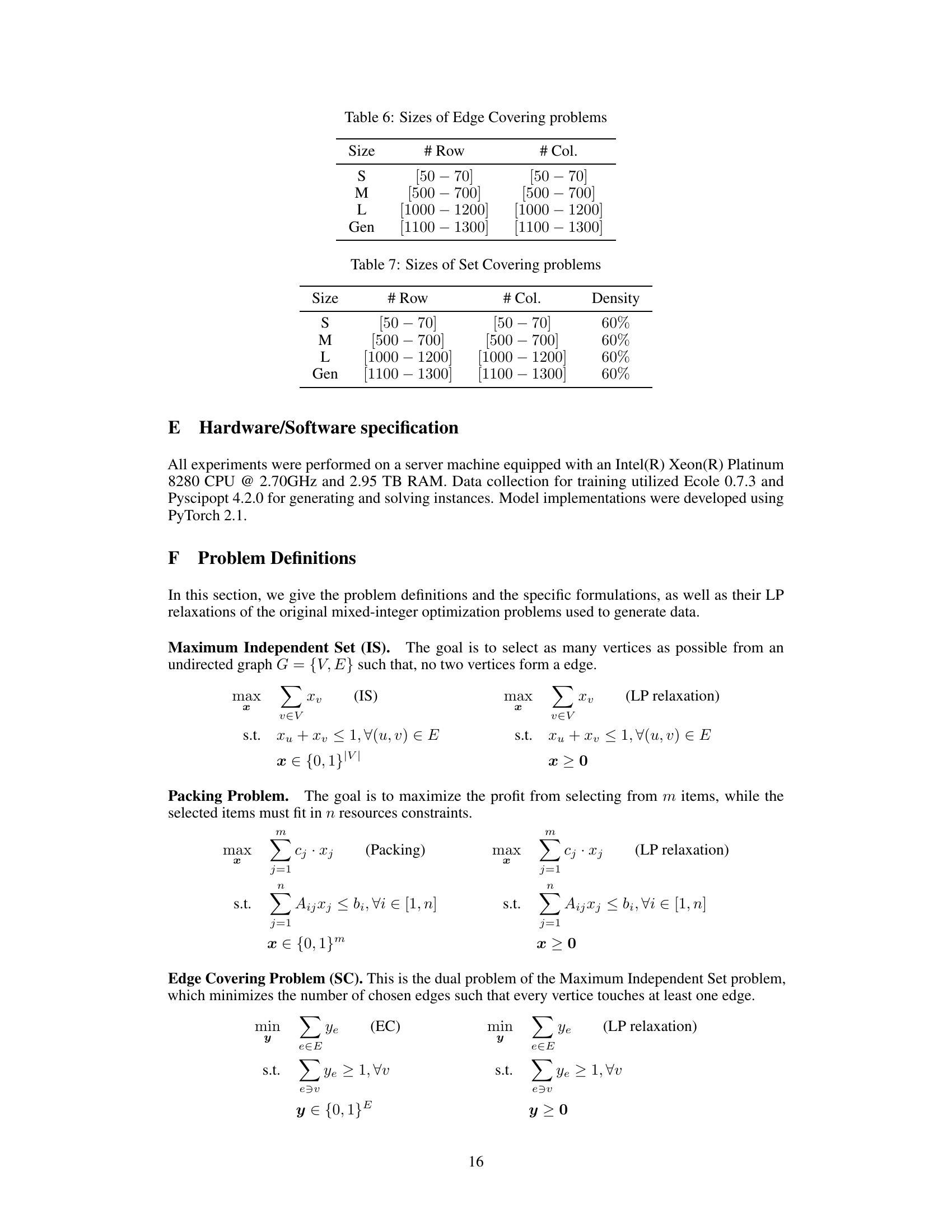
This research addresses this gap by providing a theoretical foundation for the success of smaller GNNs. The authors prove that small GNNs (polylogarithmic depth, constant width) can effectively approximate solutions for common types of LPs (packing and covering problems). They achieve this by demonstrating that GNNs can simulate gradient descent algorithms efficiently. Furthermore, a new GNN architecture, GD-Net, is introduced and shown to significantly outperform existing methods while using fewer parameters.
Key Takeaways#
Why does it matter?#
This paper is crucial for researchers in optimization and machine learning because it bridges the gap between theoretical and practical observations regarding the effectiveness of Graph Neural Networks (GNNs) in solving Linear Programming (LP) problems. It provides a theoretical foundation for why small-size GNNs are surprisingly efficient at solving LPs, paving the way for more efficient and parameter-friendly machine learning approaches to optimization. This has implications for various application domains that involve large-scale LPs. The introduction of the GD-Net architecture further contributes to the practical applicability of this work, offering researchers a novel GNN model for achieving higher performance.
Visual Insights#
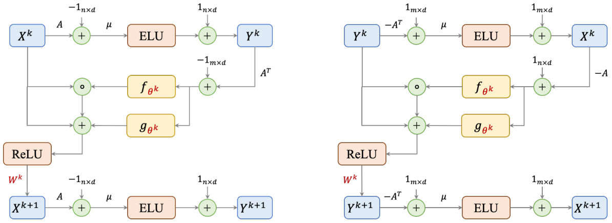
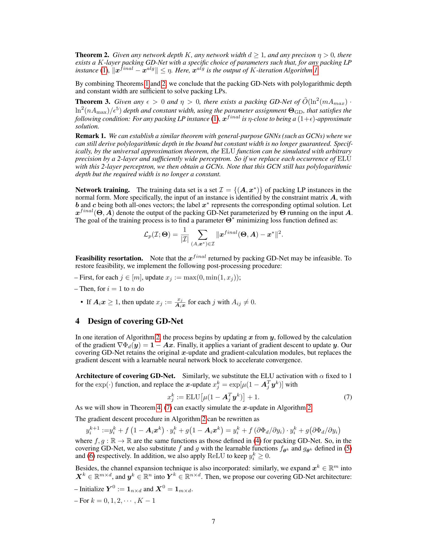
🔼 This figure shows the architecture of a single layer in both packing and covering GD-Nets. The left side illustrates the packing GD-Net, and the right side shows the covering GD-Net. Both architectures consist of several blocks including matrix multiplication with A or A transpose, addition of bias terms, ELU activation functions, learnable functions (fθk and gθk) represented by neural networks, ReLU activation, and matrix multiplication with learnable weight matrices (Wk). The learnable parameters are highlighted in red, indicating the parts of the network that are trained during the learning process. The diagrams depict the flow of information through the network, showing how the input features (Xk and Yk) are processed to generate the output features (Xk+1 and Yk+1) in a single layer. Each layer represents one iteration of the gradient descent algorithm that the GD-Net simulates.
read the caption
Figure 1: The architectures of a single layer in packing (left) and covering (right) GD-Nets. Learnable parameters are colored in red.
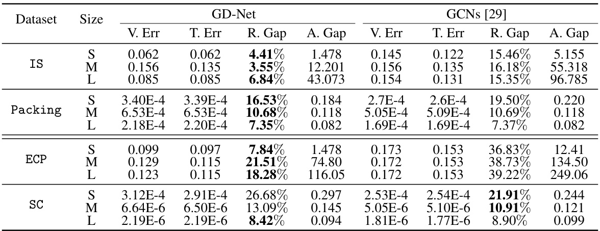
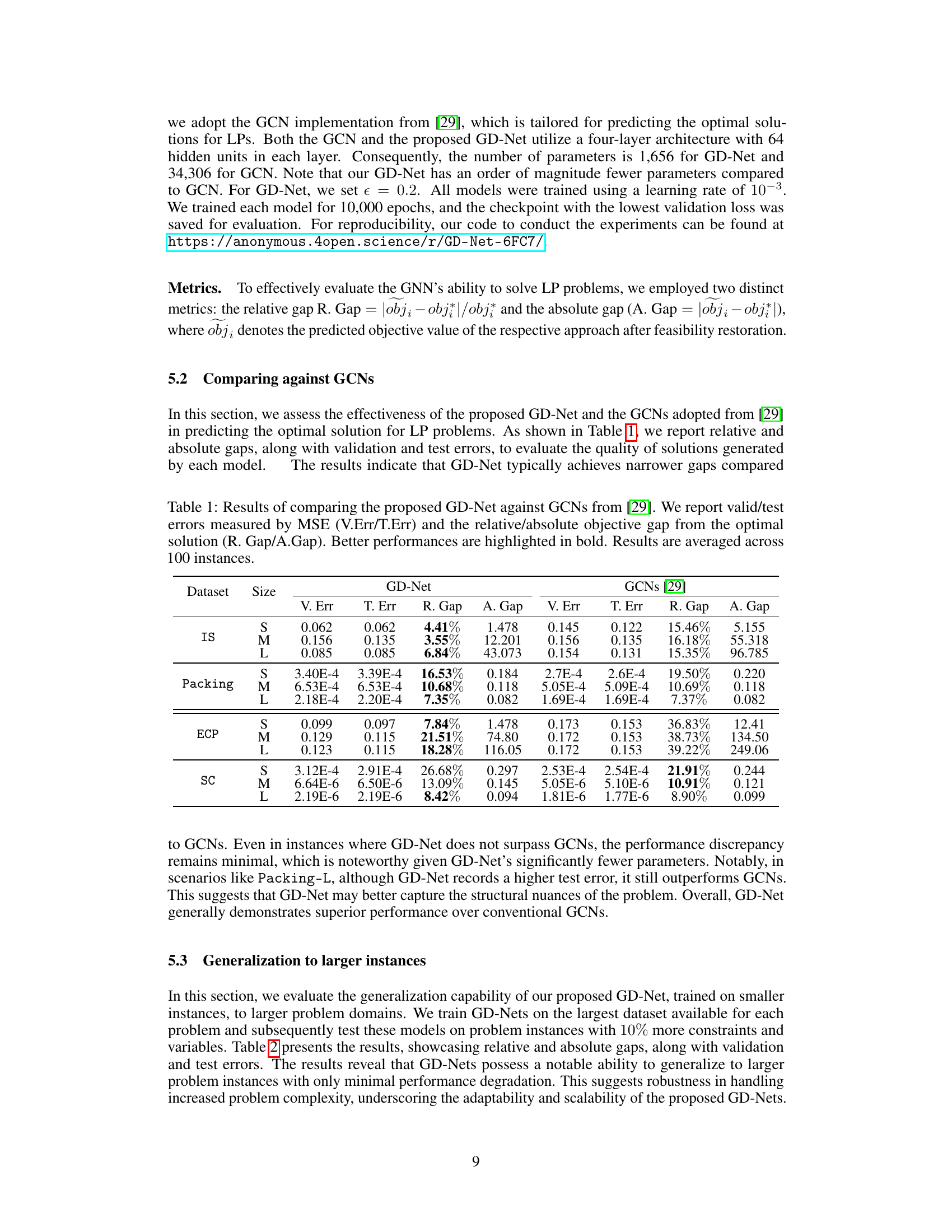
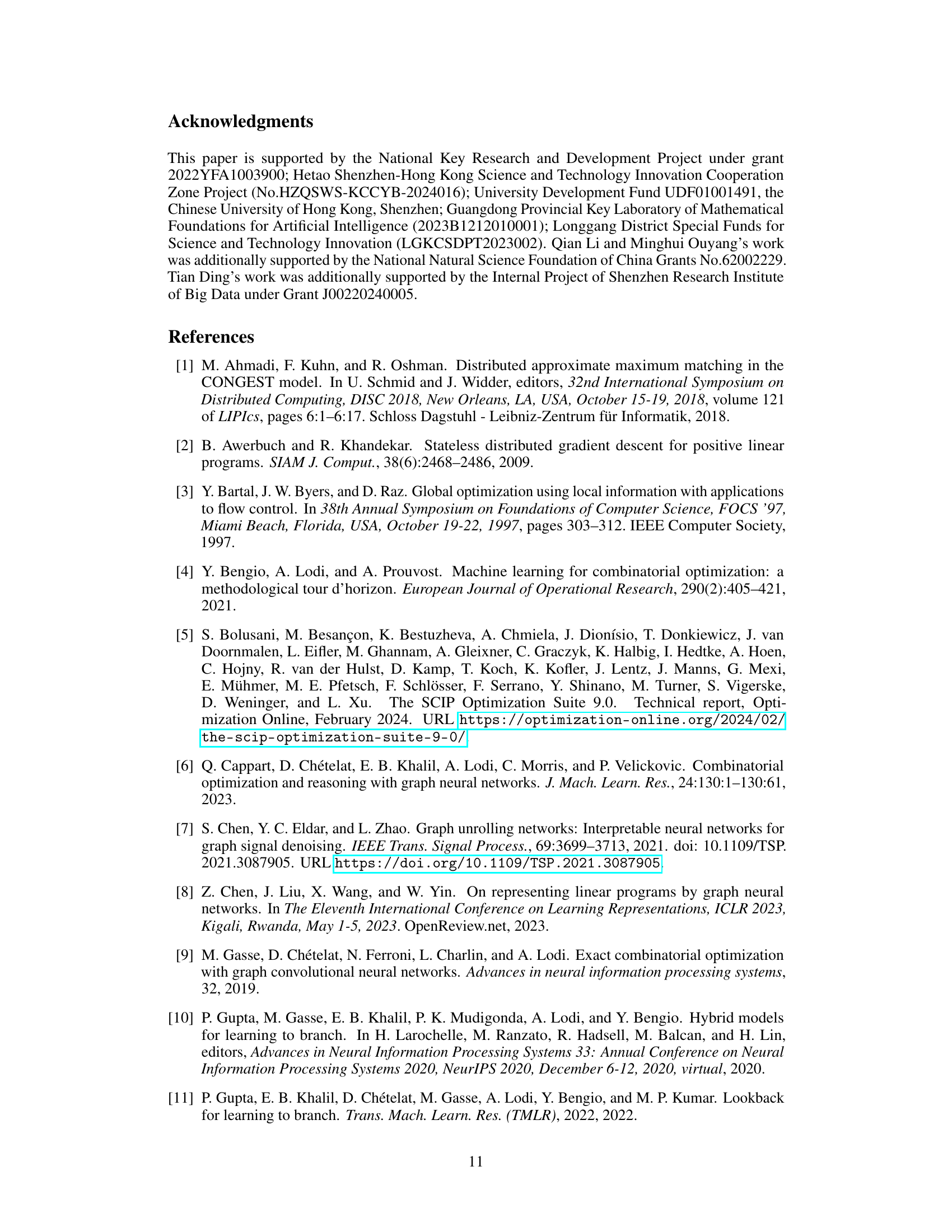
🔼 This table compares the performance of the proposed GD-Net model against GCNs from a previous study [29] across four datasets (IS, Packing, ECP, SC) and three sizes (S, M, L) of problem instances. The comparison is based on several metrics: validation error (V.Err), test error (T.Err), relative gap (R.Gap) indicating the percentage difference from the optimal solution, and absolute gap (A.Gap) showing the absolute difference from the optimal solution. Better results are highlighted in bold, and the results are averaged over 100 instances for each configuration.
read the caption
Table 1: Results of comparing the proposed GD-Net against GCNs from [29]. We report valid/test errors measured by MSE (V.Err/T.Err) and the relative/absolute objective gap from the optimal solution (R. Gap/A.Gap). Better performances are highlighted in bold. Results are averaged across 100 instances.
In-depth insights#
Small GNN Power#
The concept of “Small GNN Power” highlights the surprising effectiveness of compact graph neural networks (GNNs) in solving complex optimization problems, specifically linear programs (LPs). Traditional theoretical understanding suggests that large, deeply layered GNNs are needed for universal approximation of LP solutions. However, empirical evidence shows that smaller GNNs can achieve comparable performance, defying this expectation. This discrepancy motivates research into understanding the underlying mechanisms that enable these compact GNNs to be efficient. The “Small GNN Power” phenomenon opens the door to computationally efficient and potentially more practical applications of GNNs in optimization, particularly for resource-constrained environments. Further research could focus on characterizing the types of LPs best suited to small GNNs, identifying optimal architectural designs, and exploring whether similar principles apply to more challenging optimization problems such as mixed-integer linear programming (MILP).
GD-Net Design#
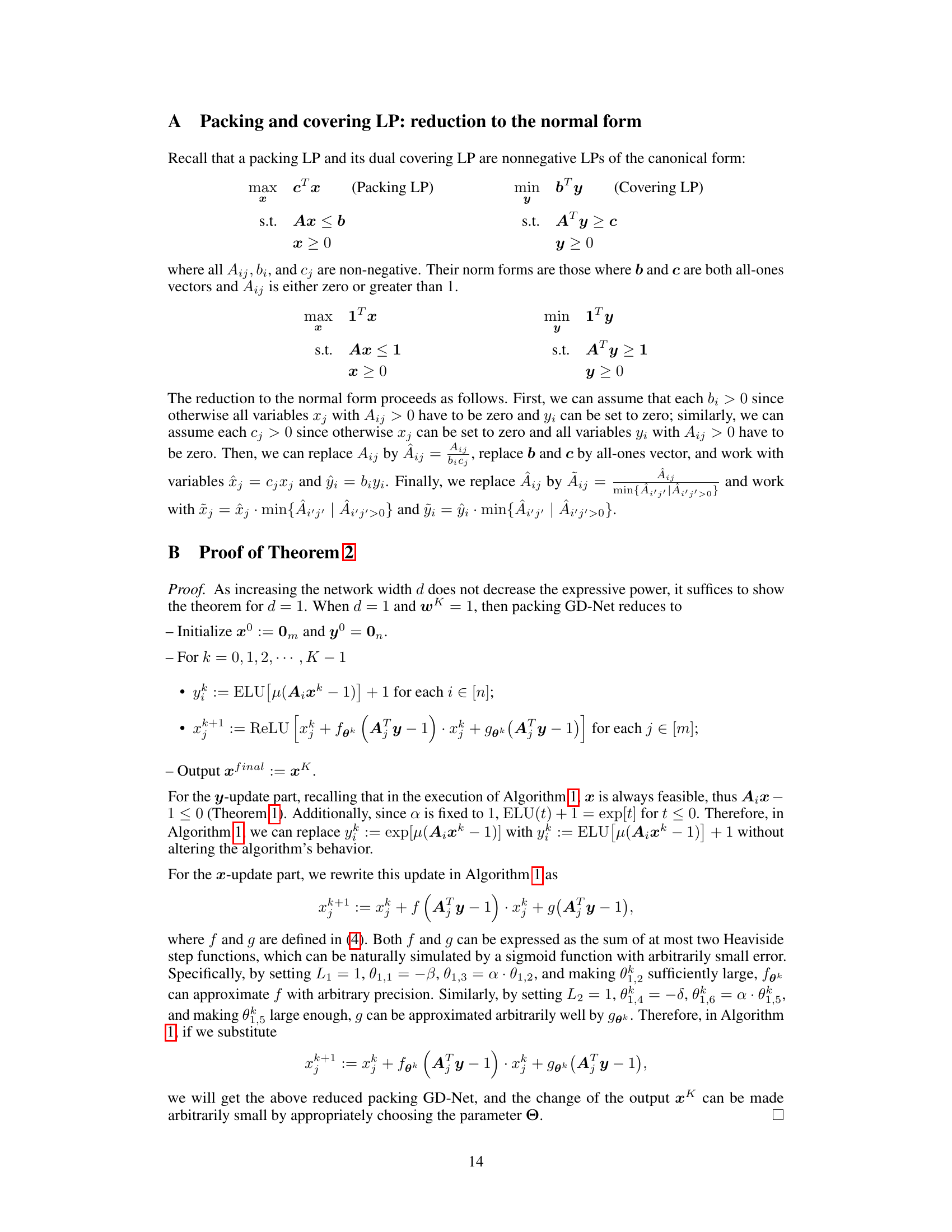
The design of GD-Net is a key contribution, leveraging the theoretical foundation established in the paper. It cleverly unrolls a variant of the Awerbuch-Khandekar gradient descent algorithm, specifically tailored for packing and covering LPs, into a novel GNN architecture. This approach directly addresses the gap between theoretical requirements for large GNNs and the practical effectiveness of smaller ones. The architecture cleverly integrates ELU activation functions to replicate the algorithm’s y-updates, ensuring precise adherence to theoretical steps. The learnable gradient descent procedure, realized using learnable functions as substitutes for the Heaviside step functions, is a crucial element, allowing the network to learn efficient updates without relying solely on pre-defined parameters. The packing GD-Net further employs a channel expansion technique to enhance its expressive power. By integrating these components, GD-Net efficiently simulates the iterative nature of the gradient descent algorithm within a GNN framework, enabling the network to learn an approximation of the optimal solution with significantly fewer parameters compared to conventional GNNs, demonstrating its superior parameter efficiency.
Theoretical Advance#
The research paper presents a significant theoretical advance by bridging the gap between theoretical and empirical findings on the application of Graph Neural Networks (GNNs) to Linear Programming (LP) problems. Prior work demonstrated that GNNs could universally approximate LP solutions, but often required large model sizes. This paper provides a rigorous proof showing that much smaller GNNs, with polylogarithmic depth and constant width, suffice for solving packing and covering LPs—two crucial subclasses of LPs. The proof leverages the ability of GNNs to simulate a gradient descent method on a carefully chosen potential function, offering a novel theoretical perspective on why small GNNs are effective in practice. This theoretical contribution is highly impactful, potentially leading to the design of more efficient and parameter-efficient GNN architectures for LP and related optimization tasks.
Empirical Validation#
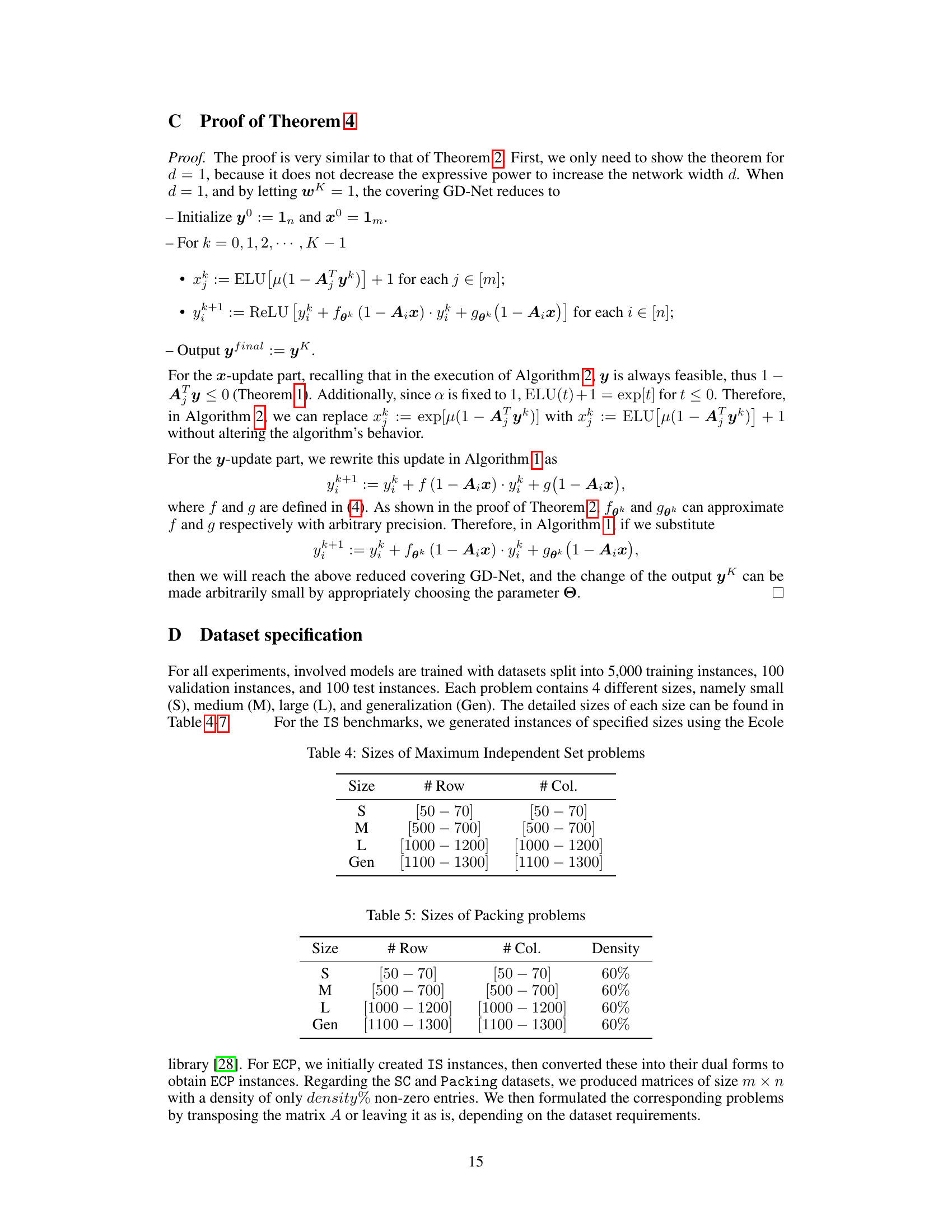
An empirical validation section in a research paper would rigorously test the proposed methods. It should present results from experiments designed to confirm the theoretical claims. This would involve selecting appropriate datasets, metrics for evaluating performance (e.g., accuracy, runtime), and comparing the proposed approach to existing baselines. A strong empirical validation would include details on the experimental setup, including dataset characteristics, parameter settings, and the statistical significance of observed differences. The section needs to demonstrate that the new approach performs as well as, or better than, alternatives in relevant scenarios. Visualizations (graphs, tables) are often beneficial for presenting the results clearly. Furthermore, a discussion of any unexpected results or limitations is crucial. It is important to focus on showing the practical impact and demonstrate the approach’s effectiveness in real-world scenarios, where applicable. A well-written empirical validation strengthens a paper’s credibility and overall contribution significantly.
Future of GNN-LP#
The future of GNN-LP (Graph Neural Networks for Linear Programming) is promising, with significant potential for advancements. Bridging the theory-practice gap is crucial; current theoretical results often require unrealistically large GNNs, while smaller GNNs perform surprisingly well in practice. Future research should focus on developing tighter theoretical bounds for smaller, more efficient GNN architectures. Exploring novel GNN architectures specifically designed to simulate iterative optimization algorithms like gradient descent will likely yield more efficient and accurate solutions. Addressing the limitations of current approaches, such as handling infeasible solutions and generalizing to broader classes of LPs, is critical. Combining GNNs with traditional LP solvers (hybrid approaches) offers a promising path towards improving the speed and robustness of LP solutions. Improving training methodologies is also essential, including developing techniques to handle noisy and incomplete data. Finally, exploring the applications of GNN-LP in new domains such as MILP and other combinatorial optimization problems will unlock additional practical value.
More visual insights#
More on tables

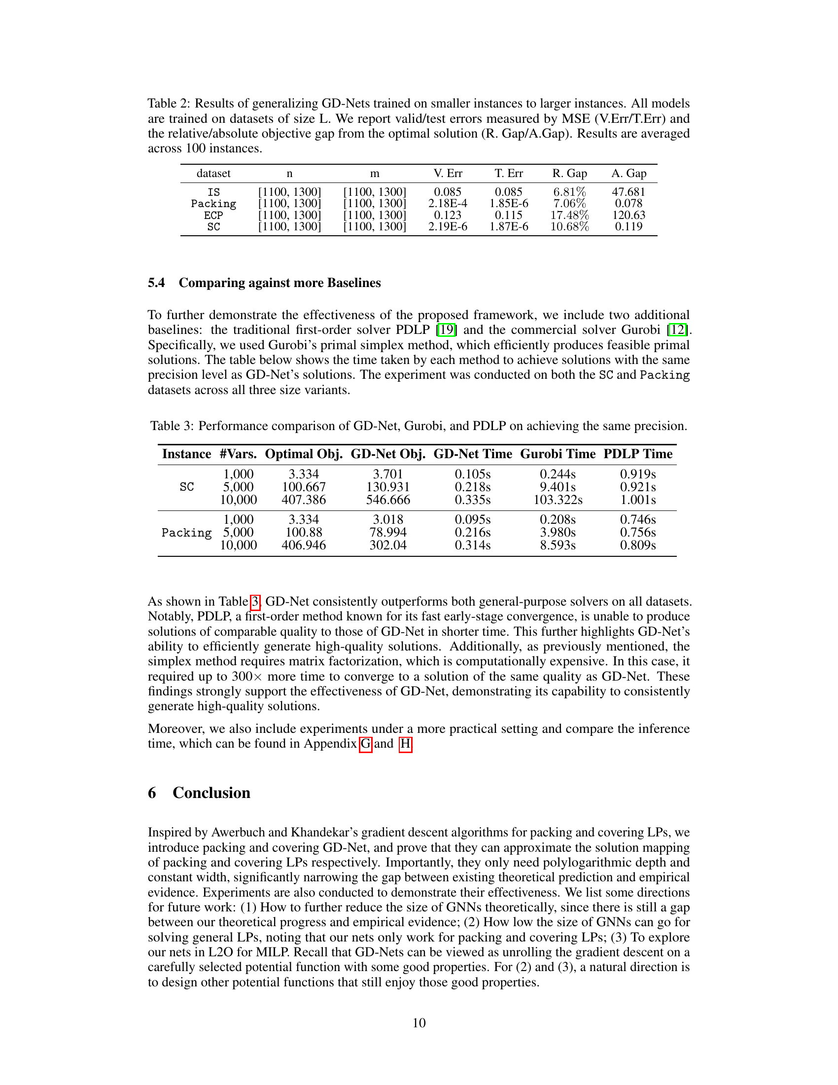
🔼 This table presents the results of evaluating the generalization capabilities of the GD-Net model. It shows how well the model trained on smaller datasets performs when tested on larger datasets. The metrics reported are the validation and test errors (mean squared error), the relative gap, and the absolute gap between the model’s predictions and the optimal solutions. The results are averaged across 100 instances for each dataset (IS, Packing, ECP, SC).
read the caption
Table 2: Results of generalizing GD-Nets trained on smaller instances to larger instances. All models are trained on datasets of size L. We report valid/test errors measured by MSE (V.Err/T.Err) and the relative/absolute objective gap from the optimal solution (R. Gap/A.Gap). Results are averaged across 100 instances.

🔼 This table compares the performance of the proposed GD-Net model against a Graph Convolutional Network (GCN) model from a previous study ([29]). The comparison is made across four different datasets (IS, Packing, ECP, SC) with varying problem sizes (small, medium, large). The evaluation metrics include the mean squared error (MSE) for validation and test sets (V.Err, T.Err), the relative gap between the predicted and optimal objective values (R.Gap), and the absolute gap (A.Gap). Better results for GD-Net are highlighted in bold.
read the caption
Table 1: Results of comparing the proposed GD-Net against GCNs from [29]. We report valid/test errors measured by MSE (V.Err/T.Err) and the relative/absolute objective gap from the optimal solution (R.Gap/A.Gap). Better performances are highlighted in bold. Results are averaged across 100 instances.
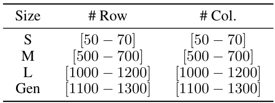
🔼 This table compares the performance of the proposed GD-Net model against a GCN model from a previous study [29] on four different datasets (IS, Packing, ECP, SC). The comparison uses several metrics: Mean Squared Error (MSE) for validation and test sets, and relative and absolute gaps between the model’s objective function value and the optimal objective value. Better performance is highlighted in bold. Results are averaged across 100 instances for each dataset and size.
read the caption
Table 1: Results of comparing the proposed GD-Net against GCNs from [29]. We report valid/test errors measured by MSE (V.Err/T.Err) and the relative/absolute objective gap from the optimal solution (R. Gap/A.Gap). Better performances are highlighted in bold. Results are averaged across 100 instances.

🔼 This table presents a comparison of the performance of the proposed GD-Net model and the GCN model from [29] on four different datasets (IS, Packing, ECP, and SC). The comparison is based on several metrics including validation error, test error, relative gap, and absolute gap. These metrics evaluate how close the models’ predictions are to the optimal solutions for linear programming problems of varying sizes. The table highlights which model performed better on each dataset and for different problem sizes.
read the caption
Table 1: Results of comparing the proposed GD-Net against GCNs from [29]. We report valid/test errors measured by MSE (V.Err/T.Err) and the relative/absolute objective gap from the optimal solution (R. Gap/A.Gap). Better performances are highlighted in bold. Results are averaged across 100 instances.

🔼 This table compares the performance of the proposed GD-Net model against a GCN model from a previous study [29] on four different datasets. The comparison uses several metrics to evaluate the quality of solutions generated by each model: mean squared error (MSE) for validation and test sets (V.Err and T.Err), relative gap between predicted objective and optimal objective (R.Gap), and absolute gap between predicted and optimal objective (A.Gap). The results are averaged over 100 instances per dataset.
read the caption
Table 1: Results of comparing the proposed GD-Net against GCNs from [29]. We report valid/test errors measured by MSE (V.Err/T.Err) and the relative/absolute objective gap from the optimal solution (R. Gap/A.Gap). Better performances are highlighted in bold. Results are averaged across 100 instances.

🔼 This table presents a comparison of the proposed GD-Net and GCNs from reference [29] for solving linear programming problems. It shows the validation and test errors (using Mean Squared Error), along with relative and absolute objective gaps from the optimal solution. The results are averaged across 100 instances and highlight GD-Net’s improved performance with significantly fewer parameters.
read the caption
Table 1: Results of comparing the proposed GD-Net against GCNs from [29]. We report valid/test errors measured by MSE (V.Err/T.Err) and the relative/absolute objective gap from the optimal solution (R. Gap/A.Gap). Better performances are highlighted in bold. Results are averaged across 100 instances.

🔼 This table compares the performance of GD-Net and GCNs on the Bipartite Maxflow problem (BMP). The table shows the objective values obtained by each model (Obj), the absolute gap (A. Gap) between the obtained objective value and the optimal objective value, and the relative gap (R. Gap) between the obtained objective value and the optimal objective value for two different problem sizes (1200 and 2000 nodes). The results show that GD-Net consistently achieves better predictions than GCNs, with smaller absolute and relative gaps. This demonstrates GD-Net’s effectiveness in solving this practical problem.
read the caption
Table 8: Comparison of GD-Net and GCN on BMP dataset

🔼 This table compares the performance of GD-Net and the Ford-Fulkerson algorithm on solving Maxflow problems with different numbers of nodes (1200 and 2000). It shows the objective value (GD-Net Obj) obtained by GD-Net, the time taken by GD-Net to achieve that objective (GD-Net Time), and the time taken by the Ford-Fulkerson algorithm to reach a solution of comparable quality (Ford-Fulkerson Time). The results highlight that GD-Net is significantly faster than the Ford-Fulkerson heuristic in achieving high-quality solutions, demonstrating its efficiency and effectiveness.
read the caption
Table 9: Comparison of GD-Net and Ford-Fulkerson on different datasets

🔼 This table compares the performance of the proposed GD-Net model against GCNs from a previous study [29] on four different datasets: IS, Packing, ECP, and SC. The performance is evaluated using mean squared error (MSE) for validation and test sets (V.Err/T.Err), and relative and absolute objective gaps (R.Gap/A.Gap) compared to the optimal solution. The table shows that GD-Net generally achieves better performance or comparable performance with significantly fewer parameters.
read the caption
Table 1: Results of comparing the proposed GD-Net against GCNs from [29]. We report valid/test errors measured by MSE (V.Err/T.Err) and the relative/absolute objective gap from the optimal solution (R.Gap/A.Gap). Better performances are highlighted in bold. Results are averaged across 100 instances.
Full paper#
