TL;DR#
DeepFake detection struggles with generalizing to unseen forgeries. Current methods primarily focus on spatial features, overlooking the frequency domain which contains important forgery traces. This limits the learning of generic forgery characteristics, impacting model accuracy and reliability.
FreqBlender addresses this by integrating frequency knowledge into the process of generating synthetic training data (pseudo-fake faces). It uses a Frequency Parsing Network to isolate frequency components related to forgery traces, blending them with real face frequencies. A dedicated training strategy addresses the lack of ground truth for frequency components. Experiments demonstrate that FreqBlender significantly improves DeepFake detection accuracy, especially across datasets, and complements existing methods.
Key Takeaways#
Why does it matter?#
This paper is important because it proposes a novel method to enhance DeepFake detection by leveraging frequency knowledge, a previously unexplored area. This significantly improves the generalization of existing DeepFake detection models and offers a new plug-and-play strategy for other methods. The adaptive frequency parsing network is a significant contribution, and the training strategy is also valuable for researchers dealing with similar problems where ground truth is not readily available. The results demonstrate the efficacy of the method on various datasets, opening new avenues for research in the field of DeepFake detection and multimedia forensics.
Visual Insights#

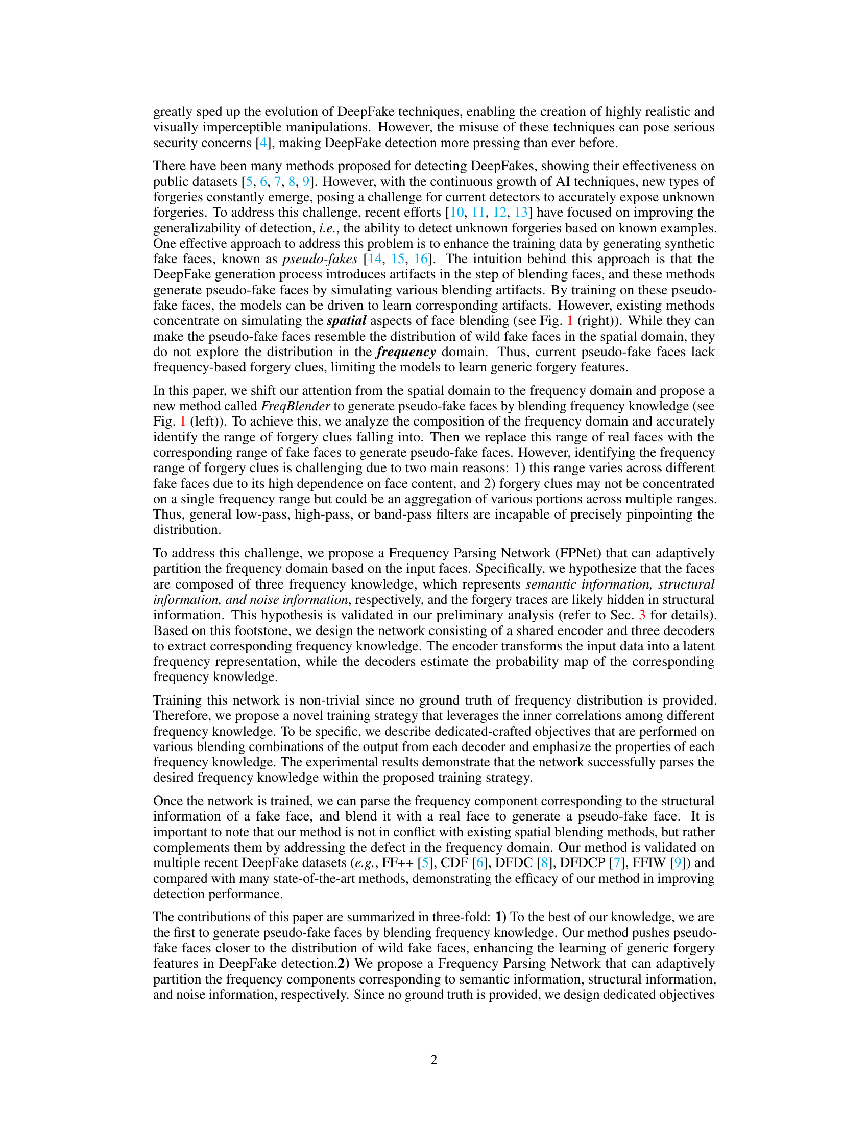
🔼 This figure illustrates the core concept of the FreqBlender method. The left side shows how the method blends frequency components from real and fake faces to create pseudo-fake faces that mimic the distribution of real-world deepfakes. This is in contrast to existing methods that primarily use spatial blending (shown on the right). The figure highlights the key difference: FreqBlender operates in the frequency domain, while traditional methods work in the spatial domain. This frequency-domain approach allows FreqBlender to generate pseudo-fakes with more realistic forgery traces, improving the generalization of deepfake detection models.
read the caption
Figure 1: Overview of our method. In contrast to the existing spatial-blending methods (right part), our method explores face blending in frequency domain (left part). By leveraging the frequency knowledge, our method can generate pseudo-fake faces that closely resemble the distribution of wild fake faces. Our method can complement and work in conjunction with existing spatial-blending methods.

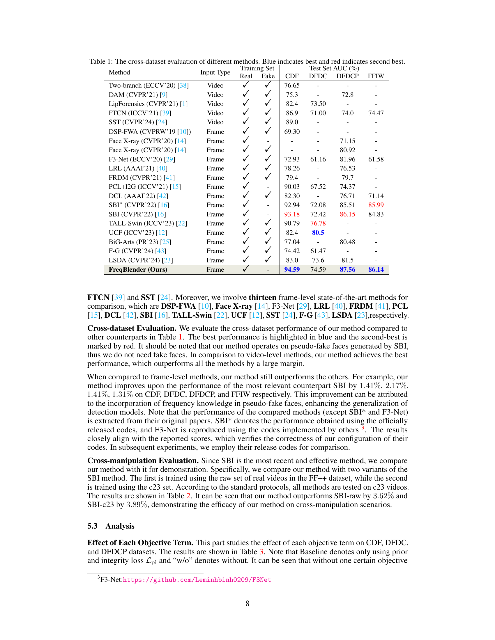
🔼 This table compares the performance of FreqBlender against several state-of-the-art DeepFake detection methods across multiple datasets (CDF, DFDC, DFDCP, FFIW). It shows the Area Under the Curve (AUC) scores for each method on each dataset. The AUC is a metric used to evaluate the performance of a binary classification model. The table highlights the best and second-best performing methods for each dataset, indicating the relative strengths of each approach in different scenarios and datasets. This demonstrates the generalization ability of the various methods.
read the caption
Table 1: The cross-dataset evaluation of different methods. Blue indicates best and red indicates second best.
In-depth insights#
FreqDomain Blending#
FreqDomain Blending, as a concept, offers a novel approach to generating synthetic training data for DeepFake detection. Instead of the typical spatial domain blending, which manipulates pixel values directly, this technique operates in the frequency domain, modifying the frequency components of images. This is significant because forgery traces often manifest as specific frequency patterns, which spatial methods might miss. By focusing on frequency blending, the method potentially captures more subtle forgery artifacts, thus improving the robustness and generalization capability of the resulting DeepFake detection models. The core challenge lies in identifying and isolating frequency components directly related to forgery, as opposed to those conveying semantic information. A dedicated network architecture and training strategy are needed to learn this mapping without ground truth labels for frequency components, requiring innovative loss functions for effective learning. The results would indicate enhanced detection performance on unseen DeepFakes due to the model’s ability to learn more comprehensive and robust forgery signatures.
FPNet Architecture#
The architecture of the Frequency Parsing Network (FPNet) is a crucial aspect of the FreqBlender method for generating pseudo-fake faces. FPNet’s design centers around a shared encoder and three distinct decoders, each specialized to extract specific frequency components: semantic, structural, and noise. The encoder processes the input face image to create a latent representation in the frequency domain. This latent representation then feeds into the three decoders. Each decoder uses a series of convolutional and PixelShuffle layers to adaptively partition the frequency components, generating probability maps that indicate the likelihood of each frequency component being present at each location in the frequency domain. The novelty lies in the adaptive partitioning and the training strategy, which doesn’t rely on ground truth frequency labels. Instead, the training process leverages internal correlations between different frequency components using carefully designed loss functions, including facial fidelity loss, authenticity-determinative loss, and quality-agnostic loss. This innovative architecture effectively leverages the frequency domain’s unique characteristics in generating realistic and diverse pseudo-fake faces that bridge the distribution gap between real and fake faces in the frequency domain, thus improving deepfake detection accuracy.
Training Strategy#
The effectiveness of a deepfake detection model heavily relies on the quality and diversity of its training data. A crucial aspect often overlooked is the frequency domain representation of facial images. A sophisticated training strategy should consider the challenges of blending frequency components without ground truth labels. This would necessitate a multi-objective training approach, potentially incorporating techniques like self-supervision to leverage inner correlations between different frequency bands (semantic, structural, noise). The strategy must address the non-trivial nature of learning from frequency data, likely involving innovative loss functions that capture the relationship between frequency components and forgery traces. It is important to ensure the training process is stable and generalizable, capable of generating pseudo-fake faces that resemble the statistical distribution of real-world deepfakes. The adaptive partitioning of frequency components is another critical aspect, potentially utilizing a neural network to dynamically identify forgery-relevant regions.
Cross-dataset Results#
Cross-dataset evaluation is crucial for assessing the generalizability of deepfake detection methods. A model performing well on one dataset might fail on another due to differences in data distribution, generation techniques, and image characteristics. Therefore, reporting cross-dataset results is essential to demonstrate robustness and real-world applicability. Analyzing these results helps understand which aspects of the models generalize well and where they fail. Key insights might involve identifying dataset-specific biases or highlighting the effectiveness of certain features across diverse datasets. The cross-dataset results section should thoroughly detail these findings, showing AUC scores or similar metrics, alongside statistical significance measures. This rigorous analysis would reveal whether the model learns generalizable deepfake traces or overfits to specific dataset artifacts, informing future research directions. Ultimately, the success of a deepfake detection model lies not only in its performance on individual datasets but, more importantly, its ability to generalize across unseen data. A robust and reliable detection system requires consistently high performance on multiple diverse datasets.
Future Enhancements#
Future enhancements for FreqBlender could explore several promising avenues. Improving the Frequency Parsing Network (FPNet) is crucial; a more robust architecture that handles diverse face characteristics and forgery techniques is needed. Investigating different frequency blending strategies beyond simple additive blending might significantly improve pseudo-fake realism. Exploring frequency components beyond semantic, structural, and noise, perhaps incorporating temporal information or subtle artifacts unique to specific DeepFake methods, is key. Furthermore, exploring alternative training paradigms beyond the proposed strategy, such as adversarial training, could enhance the network’s robustness and generalizability. Finally, extending the method to videos presents a significant challenge and opportunity, requiring efficient handling of temporal dependencies and the potential for more sophisticated forgery techniques in video.
More visual insights#
More on figures

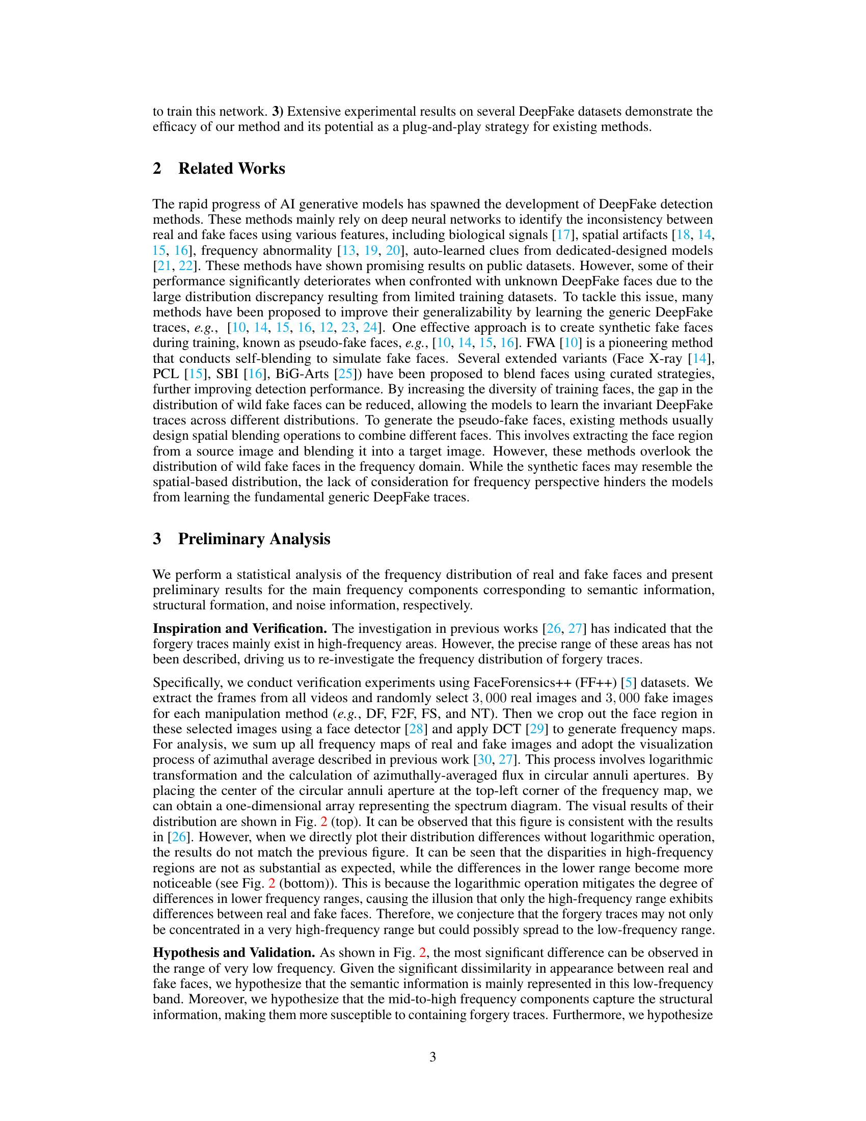
🔼 This figure shows a statistical analysis of the frequency distribution of real and fake faces. The top row presents the frequency distributions of real and fake images for four different DeepFake manipulation methods (Deepfakes, Face2Face, FaceSwap, NeuralTextures). These distributions are obtained using algorithms described in references [30] and [27]. The bottom row displays the difference between the frequency distributions of real and fake images for each manipulation method. The y-axis uses a logarithmic scale (base 2). The figure visually demonstrates that the difference in frequency distribution between real and fake faces is more prominent in lower-frequency ranges, rather than only high-frequency as previously believed.
read the caption
Figure 2: Statistics of frequency distribution. The top part shows the frequency distribution of real and fake faces using algorithms in [30, 27]. The bottom part shows the frequency difference between real and fake. The values on the vertical axis are logarithmic with 2.

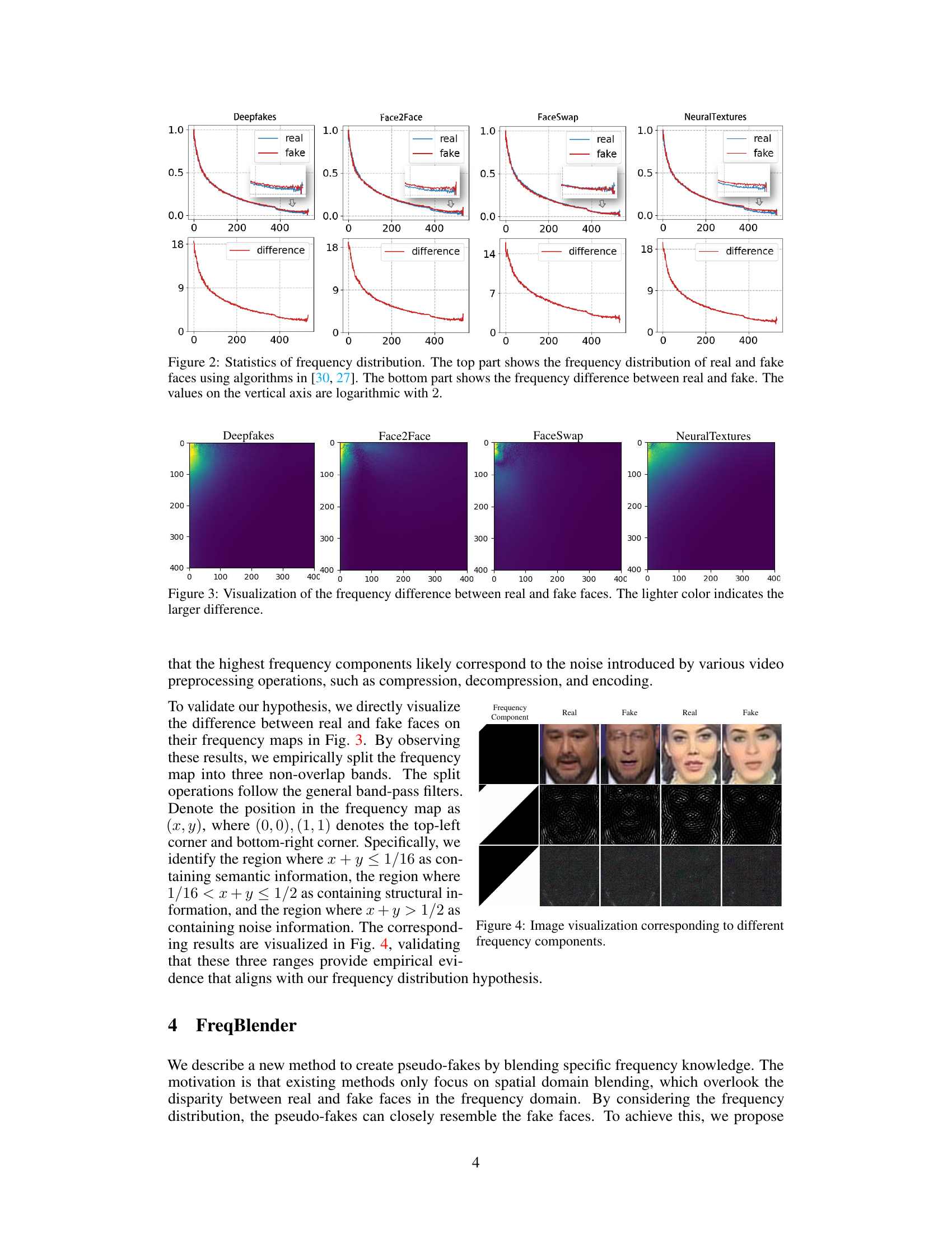
🔼 This figure visualizes the differences in frequency distribution between real and fake faces generated by four different deepfake methods: Deepfakes, Face2Face, FaceSwap, and NeuralTextures. Each subfigure represents a deepfake method, showing a heatmap of the frequency domain. Lighter colors in the heatmap indicate larger differences between the frequency distributions of real and fake faces for that method, highlighting frequency regions that are potentially indicative of forgery traces. This visualization helps support the paper’s hypothesis that forgery traces are not exclusively located in high-frequency components but also span to mid- and low-frequency ranges.
read the caption
Figure 3: Visualization of the frequency difference between real and fake faces. The lighter color indicates the larger difference.

🔼 This figure visualizes the differences in frequency components between real and fake faces generated by four different deepfake methods: Deepfakes, Face2Face, FaceSwap, and NeuralTextures. The visualization uses a heatmap to show the magnitude of the difference for each frequency component. Lighter colors represent larger differences, indicating areas where the frequency characteristics of real and fake faces differ most significantly, potentially highlighting areas containing forgery traces. The figure suggests that the differences are not uniformly distributed across all frequencies but rather are concentrated in specific frequency bands, implying that forgery artifacts are not equally prominent across the entire frequency spectrum.
read the caption
Figure 3: Visualization of the frequency difference between real and fake faces. The lighter color indicates the larger difference.

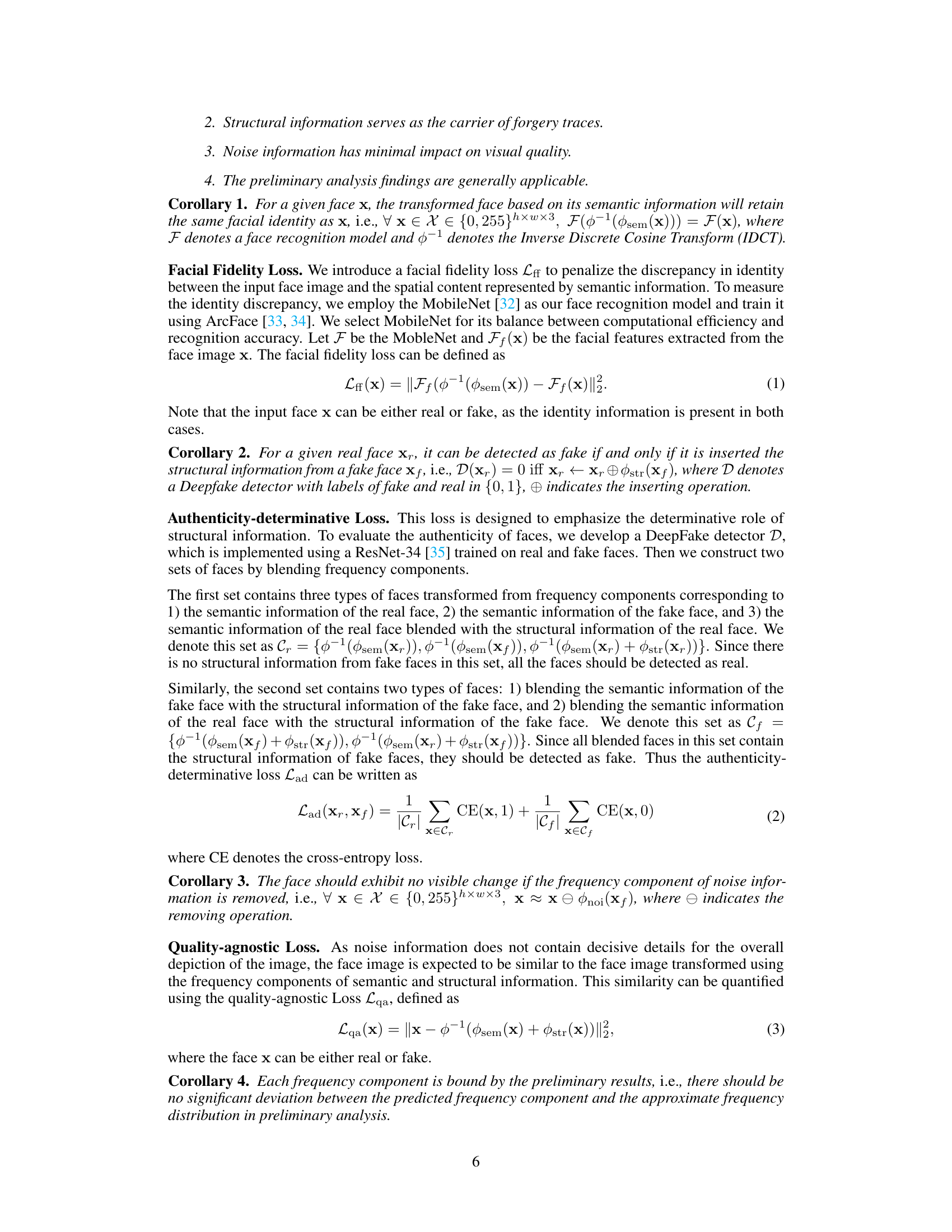
🔼 This figure illustrates the architecture of the Frequency Parsing Network (FPNet). FPNet is composed of one shared encoder and three decoders. The encoder takes an input face image and converts it to a frequency map using Discrete Cosine Transform (DCT). Three decoders then extract semantic, structural, and noise information from the frequency map. Since ground truth for frequency components isn’t available, four corollaries are used to supervise the training process. The right part of the image shows the architecture of the encoder and decoders, revealing their use of convolutional layers and PixelShuffle operations.
read the caption
Figure 5: Overview of the proposed Frequency Parsing Network (FPNet). Given an input face image, our method can partition it into three frequency components, corresponding to the semantic information, structural information, and noise information respectively. Since there is no ground truth, we propose four corollaries to supervise the training. The architecture of the encoder and decoders is shown in the right part.

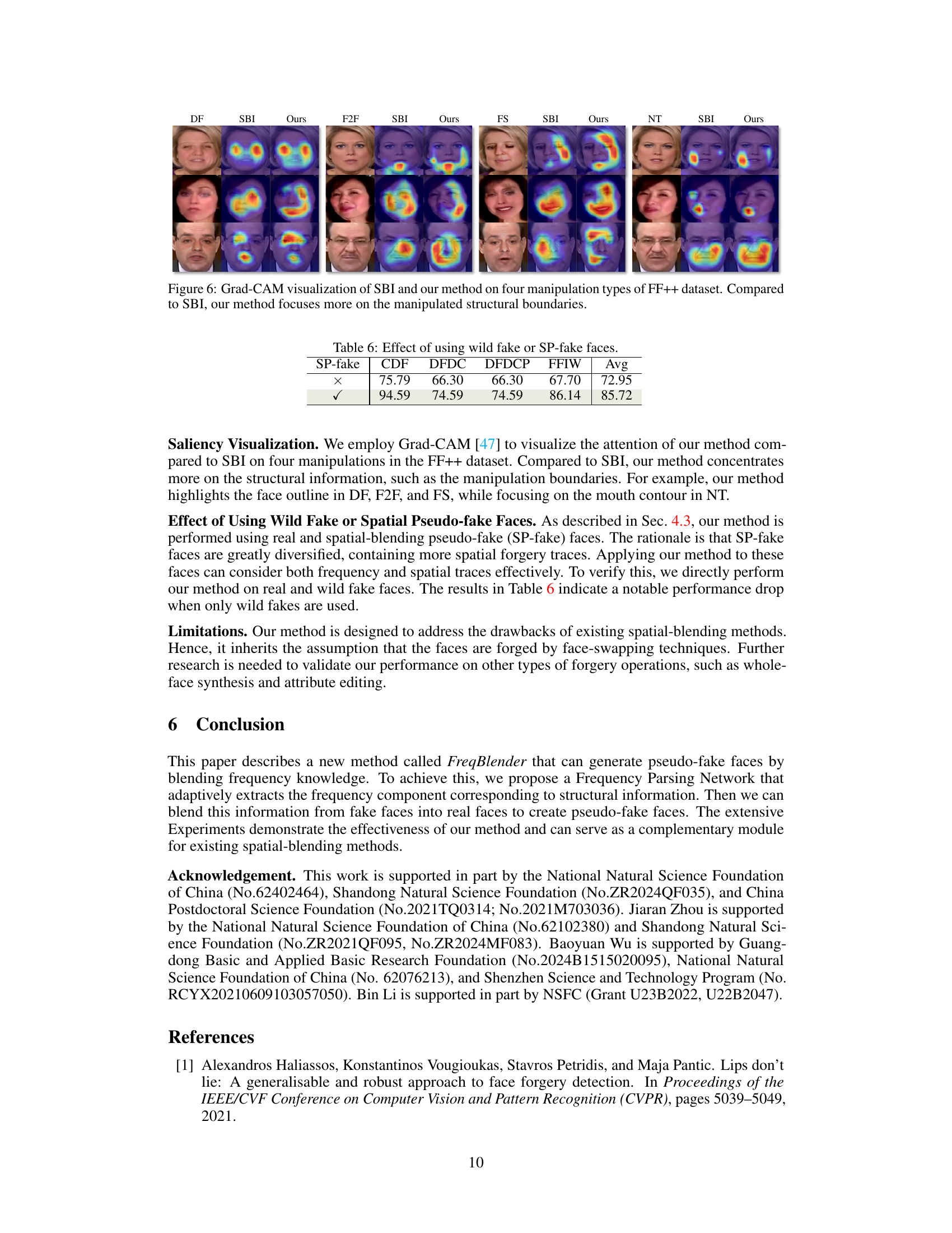
🔼 This figure shows a comparison of Grad-CAM visualizations between the SBI method and the proposed FreqBlender method. Grad-CAM is a technique used to visualize which parts of an image a neural network focuses on when making a prediction. The figure presents visualizations for four different types of face manipulations from the FaceForensics++ dataset (DF, F2F, FS, NT). Each column represents a manipulation type, and each row shows a different example image. The left image shows the visualization for the SBI method and the right for FreqBlender. The heatmaps indicate the attention areas, with warmer colors (yellow/red) representing higher attention and cooler colors (blue/purple) lower attention. The results suggest that FreqBlender focuses more on the structural boundaries of manipulated regions compared to SBI, indicating a difference in how the two methods process and interpret forgery traces.
read the caption
Figure 6: Grad-CAM visualization of SBI and our method on four manipulation types of FF++ dataset. Compared to SBI, our method focuses more on the manipulated structural boundaries.
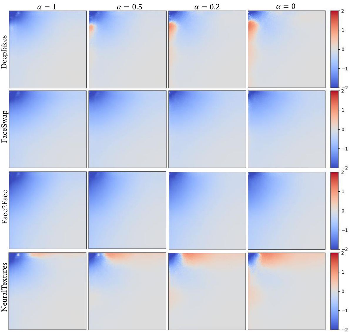
🔼 This figure visualizes the frequency difference between the proposed FreqBlender method and the ground truth frequency distribution of four types of wild fake faces (Deepfakes, FaceSwap, Face2Face, and NeuralTextures). Each cell in the figure represents one of the four types of wild fake faces. The x-axis represents the probability α of applying FreqBlender and shows four different values (α=1, 0.5, 0.2, 0). The y-axis represents the frequency component. The colormap represents the frequency difference, with red indicating a larger difference and blue indicating a smaller difference. It is shown that when α=1, the frequency distribution of the pseudo-fake faces generated by FreqBlender is closest to the ground truth distribution of wild fake faces.
read the caption
Figure 7: Heatmap visualization of the frequency difference between our method and the wild fake faces (Deepfakes, FaceSwap, Face2Face, NeuralTextures). Note that α = 0 denotes that our method is degraded to SBI [16].
More on tables

🔼 This table presents the cross-manipulation results of different DeepFake detection methods on the FF++ dataset. The methods are compared across four different manipulation techniques (Deepfakes, Face2Face, FaceSwap, and NeuralTextures). The table shows the AUC scores achieved by each method on each manipulation type, as well as the average AUC across all manipulation types. It highlights the relative performance of FreqBlender (the proposed method) against existing state-of-the-art methods (SBI-raw and SBI-c23). The results demonstrate the effectiveness of FreqBlender in improving the generalization performance of DeepFake detection models.
read the caption
Table 2: The cross-manipulation evaluation of different methods.
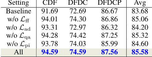
🔼 This table presents the ablation study results showing the impact of each objective term (Lff, Lad, Lqa, Lpi) on the overall performance of the FreqBlender method. The ‘Baseline’ row indicates the performance with all objective terms included. Subsequent rows show performance when removing one objective term at a time. This demonstrates the individual contribution of each objective to the overall effectiveness of the model. The results are presented in terms of AUC (%) across three datasets (CDF, DFDC, DFDCP) and an average across all three. The higher AUC percentage indicates a better performance on the task of detecting DeepFakes.
read the caption
Table 3: Effect of each objective term.

🔼 This table presents the Area Under the Curve (AUC) scores achieved by different deepfake detection methods across various datasets. Each method was tested on multiple datasets (CDF, DFDC, DFDCP, FFIW), after being trained on a single dataset (usually FF++). The table showcases the generalization ability of each method, as the differences between AUC scores across datasets highlight a model’s robustness to unseen data. Higher AUC values indicate better performance. The best and second-best results for each dataset are highlighted in blue and red, respectively.
read the caption
Table 1: The cross-dataset evaluation of different methods. Blue indicates best and red indicates second best.
🔼 This table presents the Area Under the Receiver Operating Characteristic Curve (AUC) scores achieved by various deepfake detection methods across multiple datasets. The methods are tested on four different datasets (CDF, DFDC, DFDCP, FFIW), and the table highlights the best and second-best performing methods for each dataset. The results show how well each method generalizes to unseen data, indicating its robustness and effectiveness in detecting deepfakes.
read the caption
Table 1: The cross-dataset evaluation of different methods. Blue indicates best and red indicates second best.

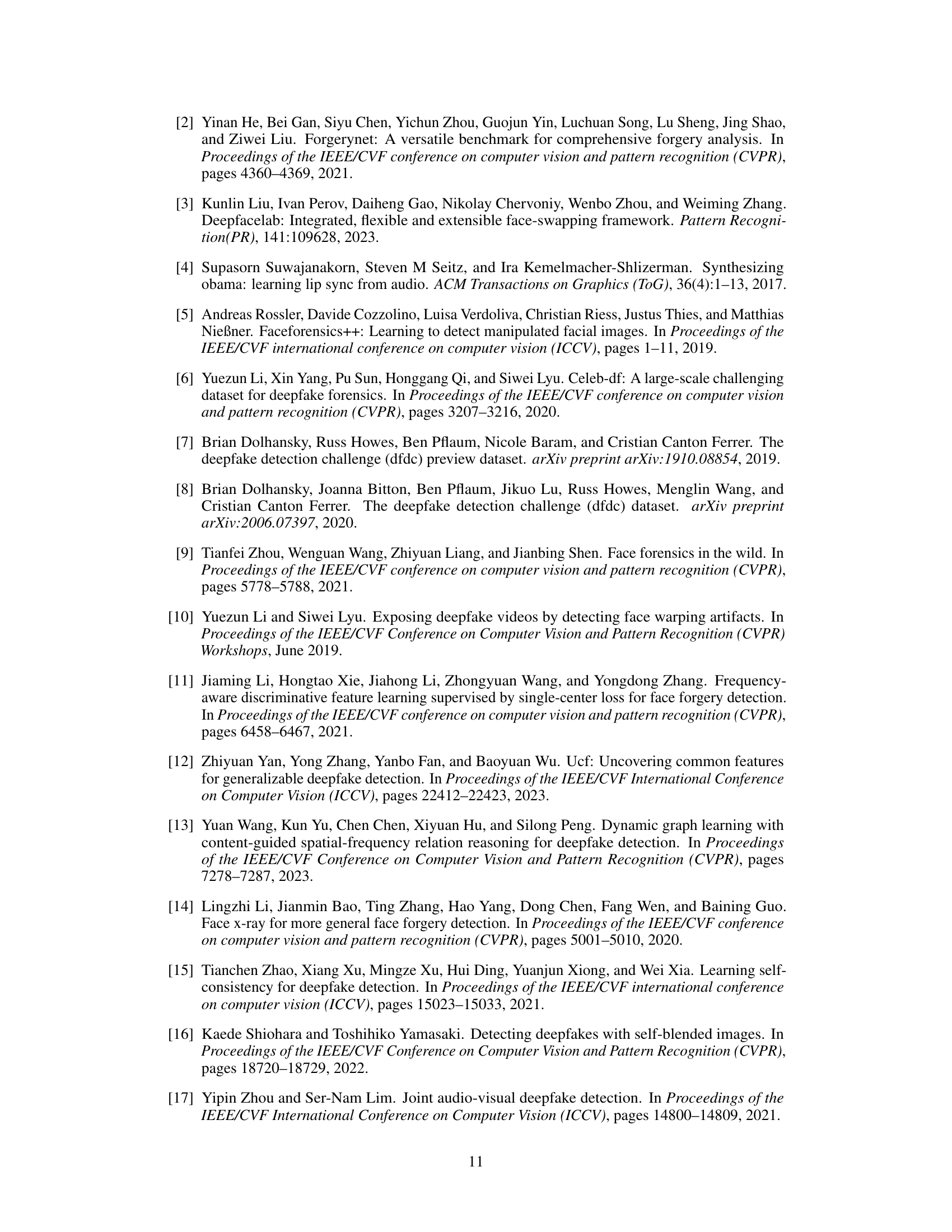
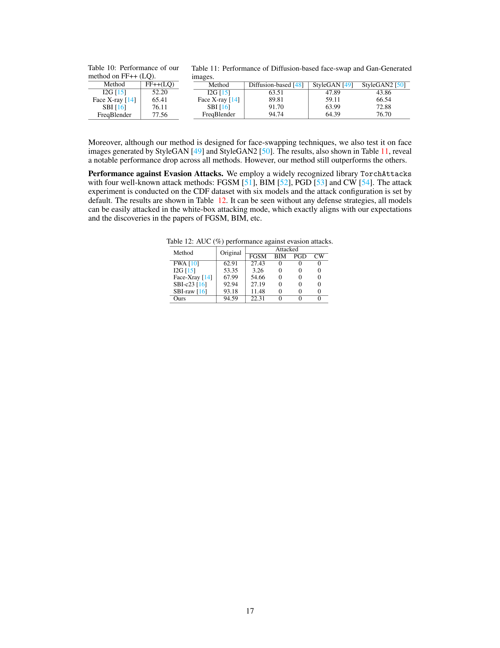
🔼 This table compares the performance of the proposed FreqBlender method using two types of pseudo-fake faces: those generated using spatial blending alone (SP-fake) and those generated using both spatial and frequency blending (indicated by a checkmark). The results show a significant improvement in detection performance across four different datasets (CDF, DFDC, DFDCP, FFIW) when using the frequency blending method. This highlights the effectiveness of incorporating frequency information into the generation of pseudo-fake data for enhancing the generalizability of DeepFake detection models.
read the caption
Table 6: Effect of using wild fake or SP-fake faces.

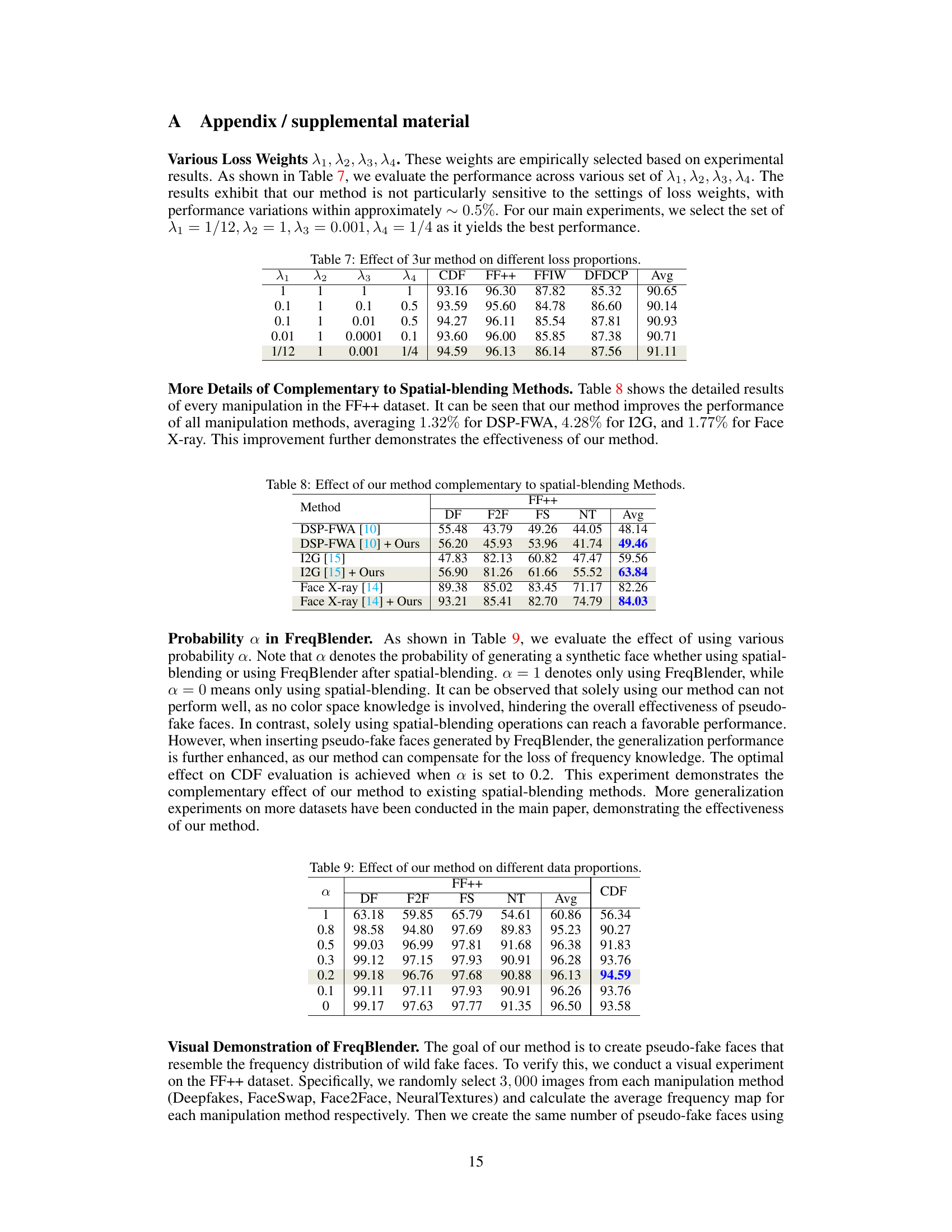
🔼 This table presents the performance of the FreqBlender method under different weight combinations for the loss functions used in training the Frequency Parsing Network. It shows the AUC scores on four DeepFake detection datasets (CDF, FF++, FFIW, and DFDCP) for various weight settings (λ1, λ2, λ3, λ4). The last column displays the average AUC across these datasets. This analysis helps determine the optimal weight combination for the loss functions, which contributes to the overall effectiveness of the FreqBlender method.
read the caption
Table 7: Effect of our method on different loss proportions.

🔼 This table presents the results of experiments where the proposed FreqBlender method is combined with three existing spatial blending methods (DSP-FWA [10], I2G [15], and Face X-ray [14]) for DeepFake detection on the FF++ dataset. The table shows the AUC (%) achieved by each of the three spatial blending methods alone and when enhanced with FreqBlender, broken down by different manipulation types (DF, F2F, FS, NT) and providing an average AUC across all manipulation types. This demonstrates the complementary nature of FreqBlender which improves the performance of the existing spatial methods.
read the caption
Table 8: Effect of our method complementary to spatial-blending Methods.

🔼 This table presents the Area Under the Curve (AUC) of various deepfake detection methods tested on several benchmark datasets. The methods are categorized by input type (video or frame) and trained on different datasets. The AUC values show the performance of each method on each test dataset. Higher AUC values represent better performance. The best and second-best results for each dataset are highlighted in blue and red, respectively.
read the caption
Table 1: The cross-dataset evaluation of different methods. Blue indicates best and red indicates second best.

🔼 This table presents the Area Under the Curve (AUC) scores achieved by various deepfake detection methods across multiple datasets (CDF, DFDC, DFDCP, FFIW). The methods are categorized into video-level and frame-level approaches, highlighting their performance on both real and fake videos from different sources. The best and second-best results for each dataset are marked in blue and red, respectively, facilitating a clear comparison of different methods’ generalization capabilities.
read the caption
Table 1: The cross-dataset evaluation of different methods. Blue indicates best and red indicates second best.

🔼 This table presents the Area Under the Curve (AUC) of different deepfake detection methods tested on several datasets. The methods are categorized into video-level and frame-level approaches. The AUC scores show the performance of each method on the different datasets, indicating how well they can distinguish between real and fake videos or images. The best and second-best performances are highlighted in blue and red, respectively. This helps to compare the generalizability and effectiveness of each method across various datasets and input types.
read the caption
Table 1: The cross-dataset evaluation of different methods. Blue indicates best and red indicates second best.
Full paper#

