↗ OpenReview ↗ NeurIPS Homepage ↗ Chat
TL;DR#
Many real-world optimization problems involve significant costs for evaluating candidate solutions. Standard Bayesian optimization, which focuses on maximizing the number of function evaluations, is insufficient for these scenarios. Current cost-aware methods often rely on complex, computationally expensive, or theoretically weak acquisition functions, limiting their practical applicability.
This paper proposes a novel acquisition function, the Pandora’s Box Gittins Index (PBGI), for cost-aware Bayesian optimization. It leverages the solution to the Pandora’s Box problem—a known optimal solution in economics—and adapts it to the Bayesian setting. The PBGI demonstrates strong empirical performance, especially in medium-to-high dimensions, often outperforming existing methods. The study further highlights the connection between cost-aware optimization and economic decision theory, opening new avenues for research.
Key Takeaways#
Why does it matter?#
This paper is important because it bridges cost-aware Bayesian optimization with economic decision theory, offering a novel, theoretically-grounded, and computationally efficient acquisition function. This addresses a critical limitation in current cost-aware Bayesian optimization methods, paving the way for more effective resource allocation in various applications. It also demonstrates strong empirical performance, even surpassing existing methods in medium-high dimensions.
Visual Insights#

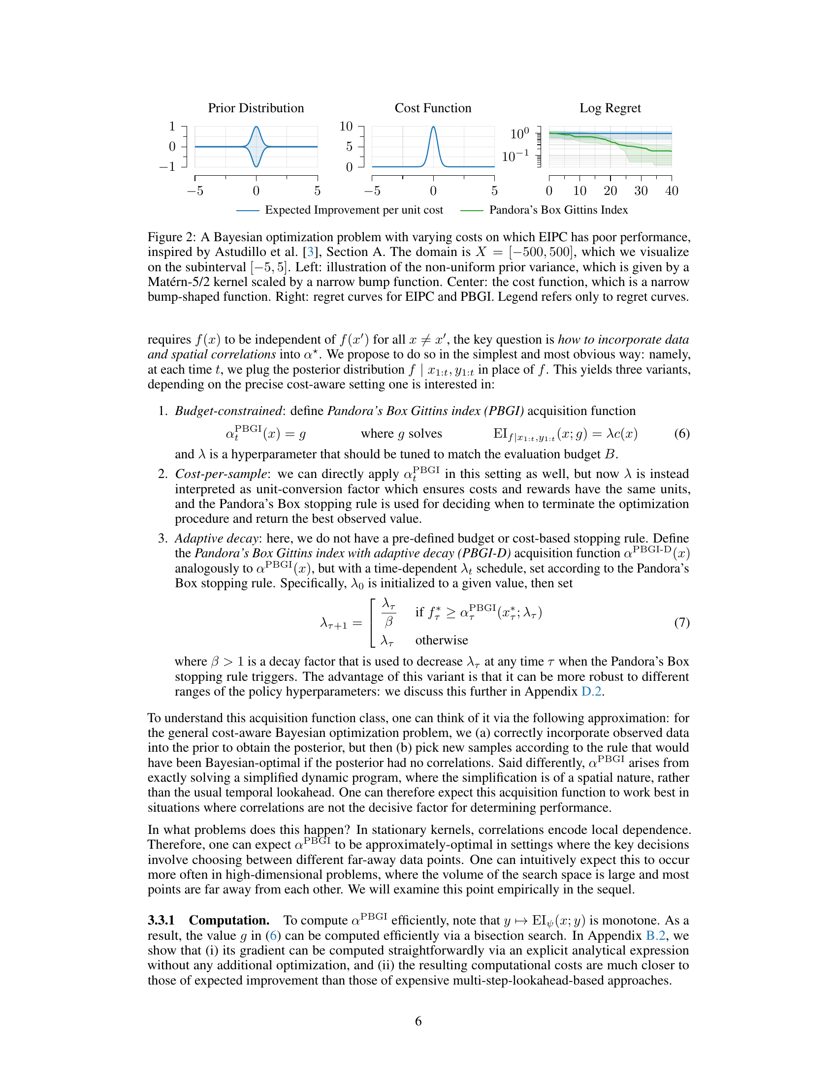
This figure illustrates the key idea of the paper by showing the connection between the Pandora’s Box problem and cost-aware Bayesian optimization. The Pandora’s Box problem is a simplified decision problem that helps to understand cost-aware Bayesian optimization. The figure shows how the Bayesian-optimal solution to the Pandora’s Box problem can be used to develop a new acquisition function for cost-aware Bayesian optimization. This new acquisition function incorporates the posterior distribution of the objective function, which makes it more effective than existing acquisition functions.
In-depth insights#
Cost-Aware BO#
Cost-aware Bayesian Optimization (BO) tackles the challenge of optimizing expensive-to-evaluate functions by explicitly considering the cost of each evaluation. Standard BO often ignores costs, leading to inefficient resource allocation. Cost-aware BO algorithms aim to find the best balance between exploration (gathering information) and exploitation (using existing knowledge) while remaining within a budget. This involves designing novel acquisition functions that consider both the expected improvement in the objective function and the cost of acquiring that improvement. The key challenge lies in developing computationally tractable acquisition functions that accurately model this cost-aware trade-off. Many proposed approaches rely on computationally expensive multi-step lookahead calculations, limiting their practical applicability. Cost-aware BO is crucial in real-world applications where evaluation costs are significant, such as in hyperparameter tuning of machine learning models, robotic control, or material design, ensuring efficient resource utilization while achieving optimal results. Further research focuses on improving the computational efficiency and theoretical guarantees of cost-aware BO algorithms.
Pandora’s Box#
The Pandora’s Box problem, a sequential decision-making model from economics, offers a unique lens for understanding cost-aware Bayesian optimization. It elegantly captures the exploration-exploitation trade-off inherent in choosing where to sample an unknown function, especially when each evaluation incurs a cost. The Bayesian-optimal solution to Pandora’s Box, expressed through the Gittins index, translates directly into a novel acquisition function for cost-aware Bayesian optimization. This acquisition function, the Pandora’s Box Gittins index (PBGI), provides a computationally efficient and theoretically grounded alternative to existing methods, particularly in medium-to-high dimensional settings. The connection between Pandora’s Box and Bayesian optimization, while previously unexplored, reveals a powerful framework for designing acquisition functions tailored to specific practical constraints, potentially extending beyond cost-aware scenarios to other challenging optimization problems.
Gittins Index#
The Gittins index, a cornerstone of bandit theory, offers a powerful framework for solving sequential decision problems under uncertainty. It provides a Bayesian-optimal solution for the Pandora’s Box problem, a model of optimal resource allocation where costs and rewards are associated with each choice. The index itself quantifies the value of exploring a particular option, balancing exploration against exploitation. In the context of Bayesian optimization, the Gittins index can be reinterpreted as an acquisition function. This work leverages this perspective, creating a new class of cost-aware acquisition functions by integrating the posterior distribution into the original Gittins index calculation. This allows for a principled and empirically effective approach to cost-aware Bayesian optimization, particularly in medium to high dimensional spaces. A key advantage is its computational tractability compared to more complex, multi-step lookahead methods. However, the approach’s performance may be impacted by the correlation structure assumed by the underlying probabilistic model, suggesting further work to consider more sophisticated correlation structures might enhance applicability.
Empirical Results#
The empirical results section of a research paper is critical for validating the proposed methods. A strong empirical results section would present results across multiple datasets or problem instances, carefully chosen to represent a range of complexities and characteristics. This helps demonstrate the generalizability of the method beyond specific, potentially favorable, test cases. The results should be presented clearly, using appropriate visualizations (e.g., graphs, tables) and statistical measures (e.g., mean, standard deviation, confidence intervals) to quantify performance. Importantly, the results should be compared against relevant baselines or state-of-the-art methods to showcase improvements or unique advantages. A thoughtful discussion of the results is essential, analyzing both strengths and weaknesses, and explaining any unexpected or counterintuitive findings. Finally, the discussion should connect the empirical findings back to the paper’s main claims and contributions, clarifying how the results support or challenge the hypotheses. Attention to detail and rigorous evaluation procedures are key to establishing the credibility and impact of the research.
Future Work#
Future research directions stemming from this Pandora’s Box Gittins Index (PBGI) for cost-aware Bayesian optimization could explore several avenues. Extending PBGI to handle more complex cost structures, such as those involving stochasticity or non-differentiability in higher dimensions, would enhance its practical applicability. Investigating the theoretical properties of PBGI, potentially establishing regret bounds or convergence rates, would provide a firmer theoretical foundation. Improving the computational efficiency of PBGI, especially for high-dimensional problems, is another crucial area. The current approach relies on numerical root-finding, which can be computationally expensive. Developing faster algorithms or approximations could significantly improve scalability. Finally, comparing PBGI against other state-of-the-art cost-aware acquisition functions on a wider range of benchmark problems, including real-world applications, would provide valuable insights into its strengths and weaknesses relative to existing methods.
More visual insights#
More on figures

This figure shows a Bayesian optimization problem with non-uniform prior variance and a narrow bump-shaped cost function. The plot on the right compares the regret (the difference between the best possible objective value and the achieved objective value) of the Expected Improvement per unit cost (EIPC) acquisition function and the Pandora’s Box Gittins Index (PBGI) acquisition function. The results illustrate that PBGI outperforms EIPC in this scenario, highlighting its improved performance in the presence of varying costs.

This figure compares the Expected Improvement (EI) acquisition function with the Pandora’s Box Gittins Index (PBGI) acquisition function. The left side shows contour plots illustrating how EI and PBGI respond to different combinations of posterior mean and standard deviation. The right side shows the performance of PBGI across different values of the hyperparameter λ. The results are from a Bayesian regret experiment with 8 dimensions.
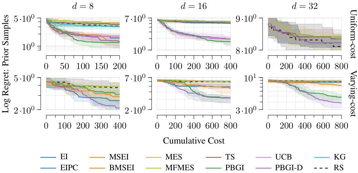
This figure shows the Bayesian regret (a measure of the optimization algorithm’s performance) for different dimensions (d = 8, 16, 32) of the problem space under both uniform and varying costs. The plots show the median regret and quartiles across multiple runs, illustrating variability. The results indicate that the Pandora’s Box Gittins Index (PBGI) and its adaptive decay variant (PBGI-D) perform comparably to or better than other state-of-the-art Bayesian optimization methods, especially in higher dimensions (d = 16, 32) and under varying costs.
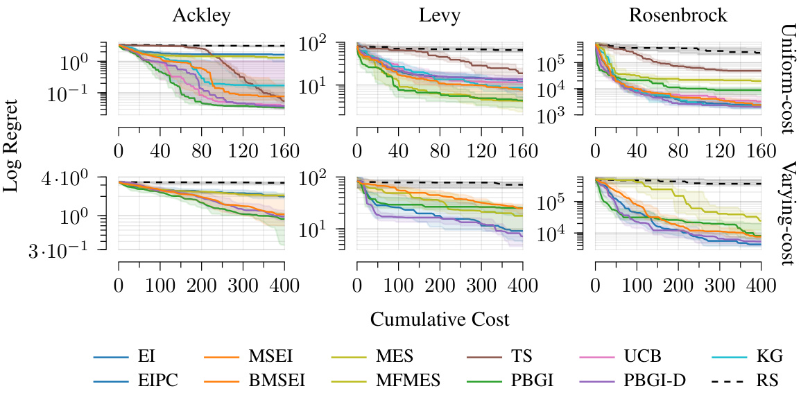
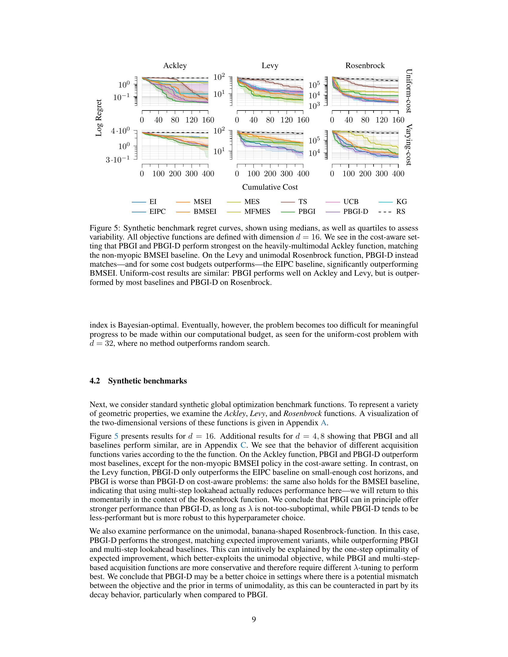
The figure compares the performance of different Bayesian optimization acquisition functions on three synthetic benchmark functions (Ackley, Levy, and Rosenbrock) with dimension d=16. The results are shown for both cost-aware and uniform-cost settings. The plots show that PBGI and PBGI-D generally perform well, especially on the Ackley function, often outperforming other baselines like EIPC and BMSEI. However, performance varied across different functions and settings.

This figure shows the empirical results on three real-world problems: Pest Control, Lunar Lander, and Robot Pushing. The plots display the best observed value against the cumulative cost for both cost-aware and uniform cost settings. The figure demonstrates that the Pandora’s Box Gittins Index (PBGI) and its variant (PBGI-D) generally outperform or match the performance of other baselines, though the performance varies across problems and settings. The results for the Robot Pushing problem highlight a potential limitation of the non-myopic BMSEI baseline in the cost-aware setting.

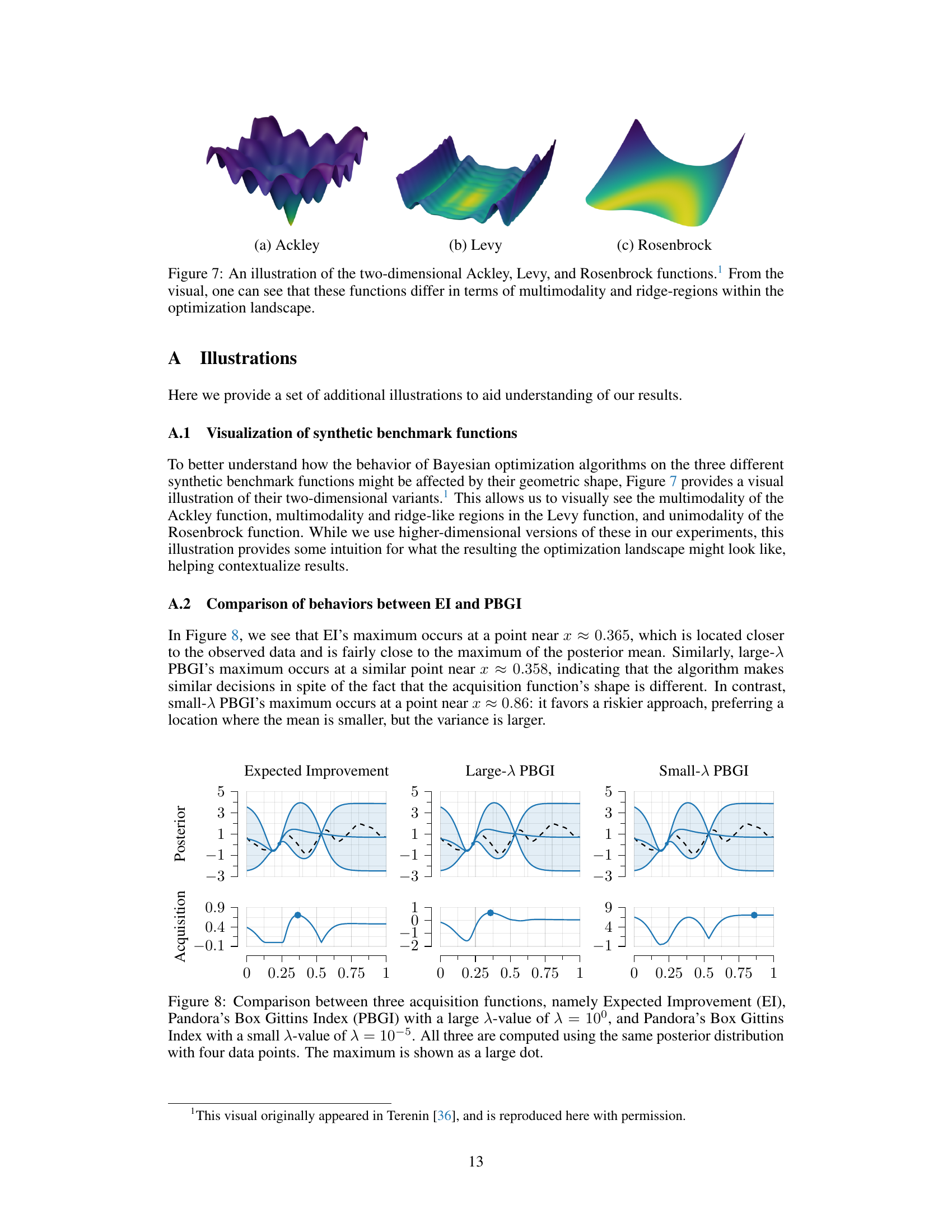
This figure shows 3D plots of the Ackley, Levy, and Rosenbrock functions in two dimensions. The plots visually demonstrate the differences in the functions’ characteristics, including the multimodality of the Ackley function (many peaks and valleys), the multimodality and ridge-like structures of the Levy function, and the unimodal (single peak) nature of the Rosenbrock function. These differences are relevant because the optimization strategies used in the paper’s experiments will perform differently depending on the function’s landscape.
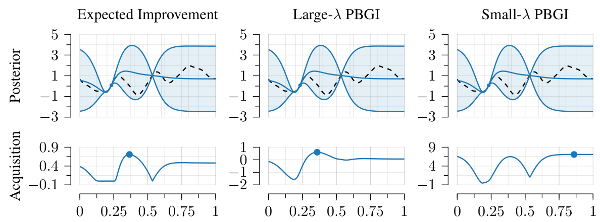
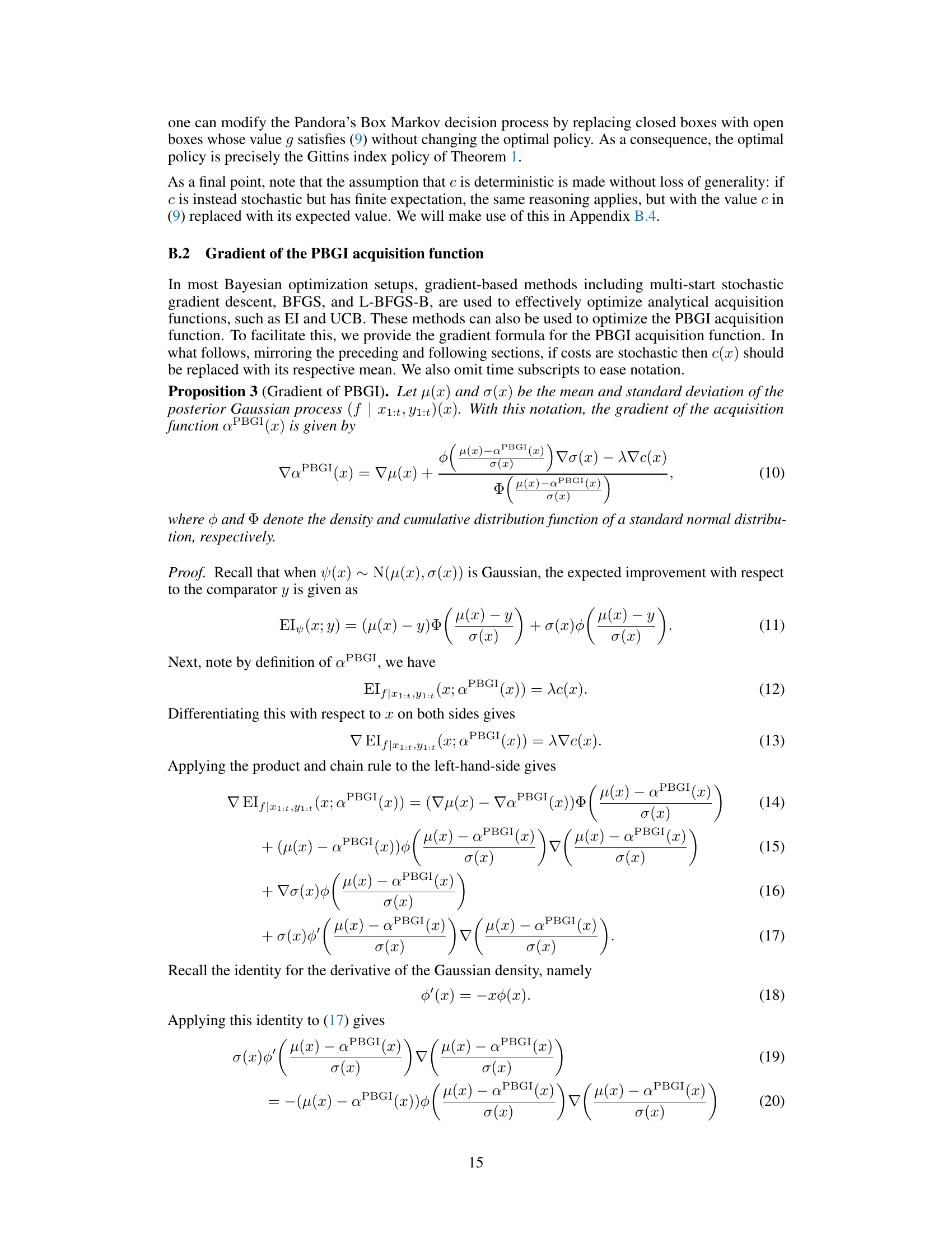
This figure compares three acquisition functions: Expected Improvement (EI), Pandora’s Box Gittins Index (PBGI) with a large λ (λ = 100), and PBGI with a small λ (λ = 10−5). All three functions are calculated using the same posterior distribution and four data points. The plot shows how the acquisition functions behave differently based on the value of λ. The top row shows the posterior distributions, and the bottom row shows the corresponding acquisition function. The large λ value leads to an acquisition function that is similar to EI, while the small λ value produces a more explorative acquisition function.

This figure shows a Bayesian optimization problem with varying costs. The left panel shows a non-uniform prior distribution. The center panel shows a cost function that is a narrow bump around 0. The right panel shows the regret curves for two algorithms: EIPC and PBGI. EIPC has poor performance compared to PBGI in this scenario because it doesn’t handle the costs effectively, and oversamples low-value, low-cost points, as discussed in the paper.
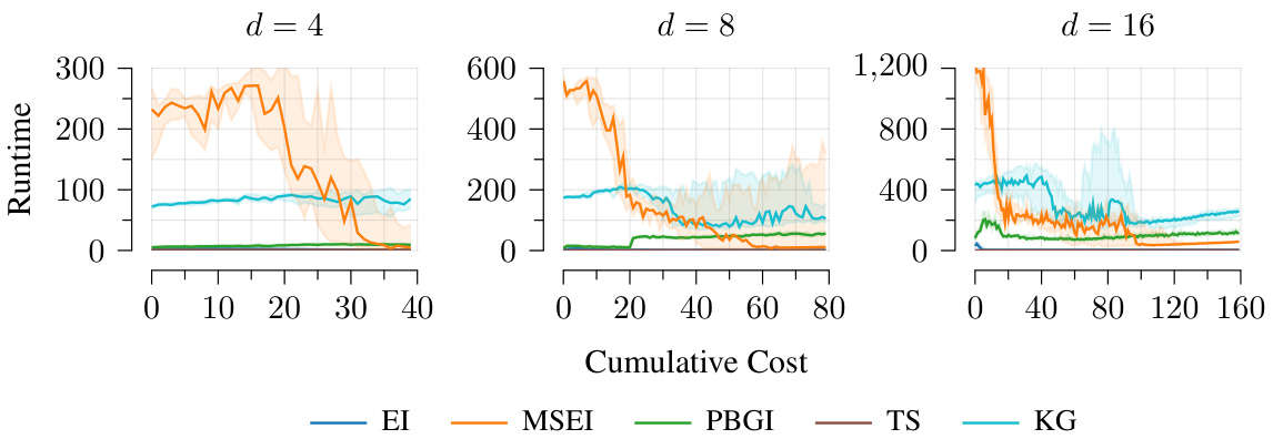
This figure compares the runtime of the Pandora’s Box Gittins Index (PBGI) acquisition function against several baselines (EI, MSEI, TS, KG) for different dimensions (d=4, 8, 16) of the Ackley benchmark function. The x-axis represents the cumulative cost, and the y-axis shows the runtime. The plot shows that while PBGI is slightly slower than EI and TS, especially in higher dimensions, it is significantly faster than the more computationally expensive methods KG and MSEI.

The figure shows the effect of hyperparameters λ₀ and β on the performance of PBGI-D in a Bayesian regret experiment with d = 8. The left plot shows median regret curves, with quartiles illustrating variability. The right plot displays the decay of λ over time for different values of λ₀ and β. The results demonstrate that performance is relatively insensitive to the choice of λ₀ and β, with small differences that are less than the variability between experiment runs with different random seeds.
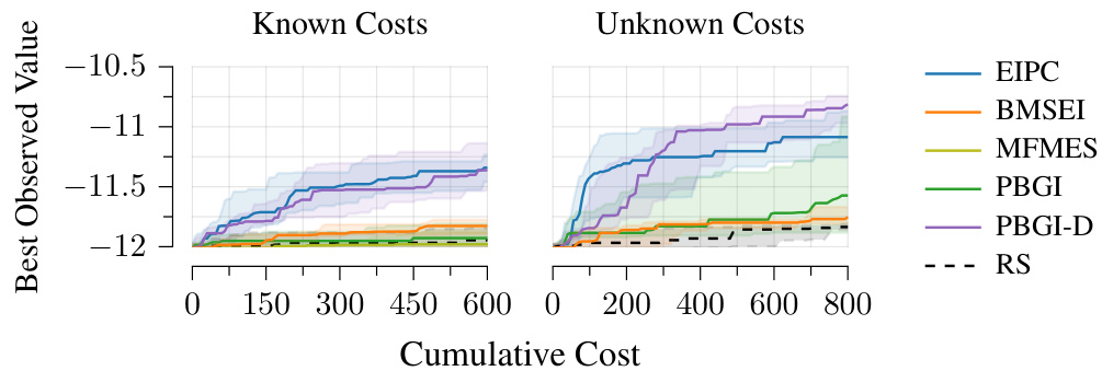
This figure compares the performance of PBGI and other acquisition functions (EI, EIPC, MSEI, BMSEI, MES, TS, MFMES, UCB, KG, PBGI-D, RS) on three empirical global optimization problems: Pest Control, Lunar Lander, and Robot Pushing. The results are shown as regret curves (median and quartiles) for both cost-aware and uniform-cost settings. PBGI shows stronger performance on Pest Control and Lunar Lander, while PBGI-D performs well on Robot Pushing along with EI and EIPC. BMSEI performs poorly on the cost-aware variant of Robot Pushing, echoing the results from the Rosenbrock function in Figure 5.
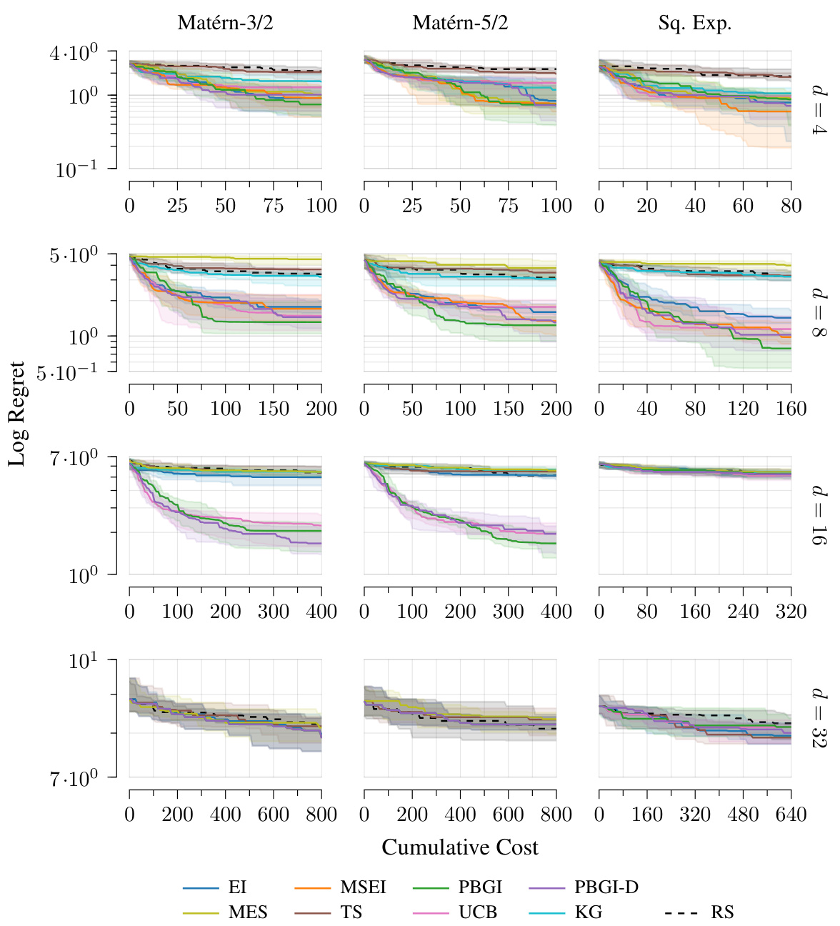
This figure compares Bayesian regret across different Gaussian process kernels (Matérn-3/2, Matérn-5/2, Squared Exponential) and various dimensions (d = 4, 8, 16, 32) in the context of uniform costs. The results show that across different kernels, the overall behavior is quite similar, although the exact transition points between ’easy’, ‘medium-hard’, and ‘very hard’ problem regimes vary. This suggests the methodology’s robustness to kernel selection.
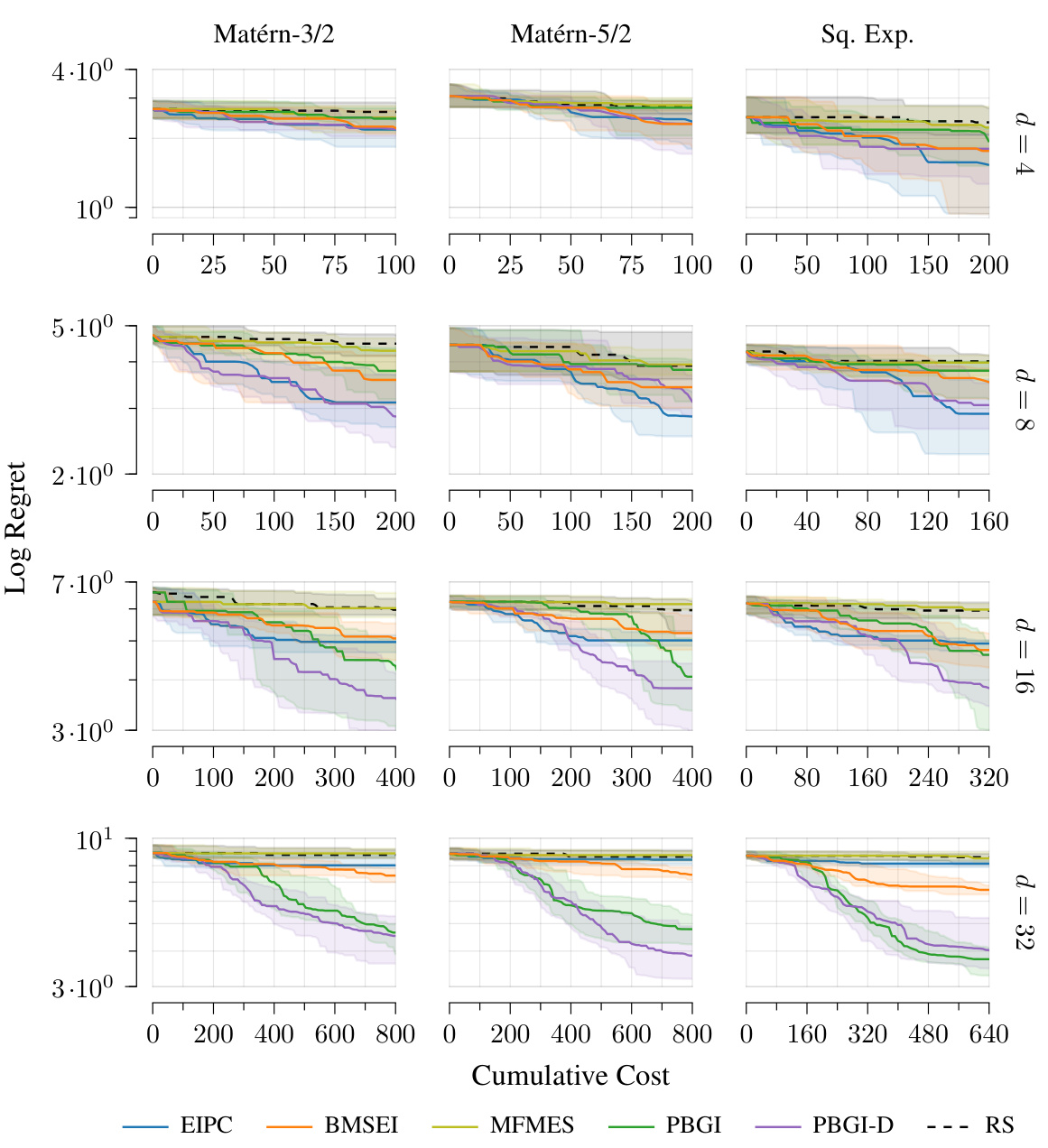
This figure compares the performance of different Bayesian optimization algorithms on problems with varying dimensionality and kernel types in a cost-aware setting. The results show that the overall behavior of the algorithms is consistent across different kernel types, but the transition points between easy, medium-hard, and very-hard problem difficulty vary depending on the specific kernel and problem dimension.
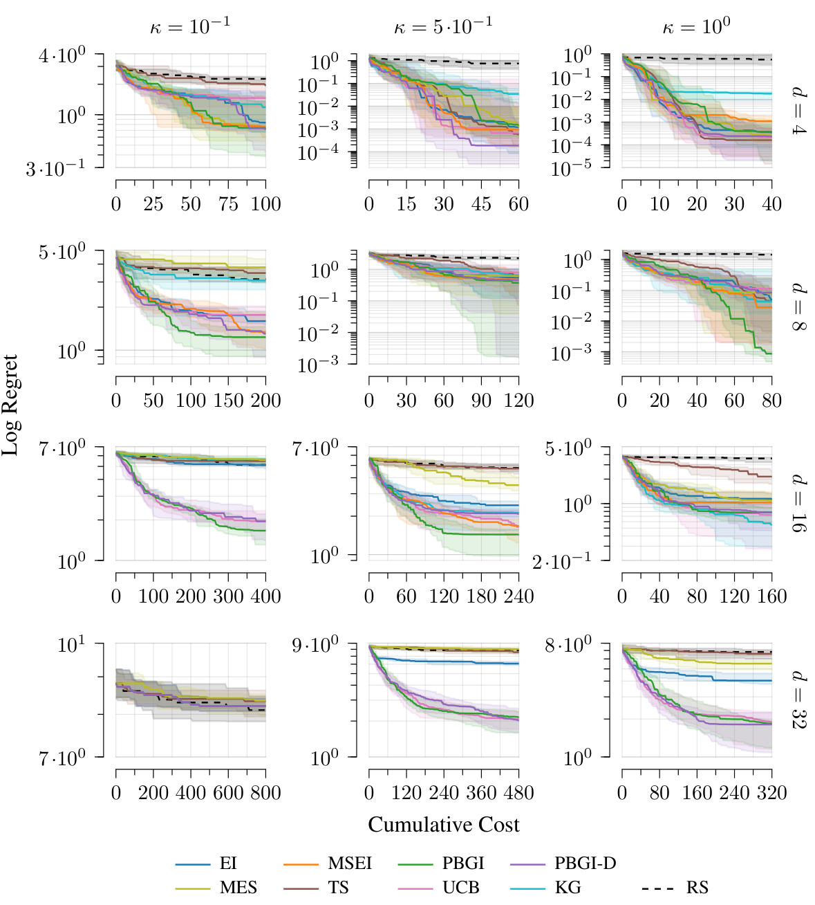
This figure shows the results of Bayesian regret experiments with different kernels (Matérn 3/2, Matérn 5/2, Squared Exponential) and various dimensions (d = 4, 8, 16, 32) in a setting without explicit costs. The plots illustrate how the regret changes over cumulative cost for multiple algorithms. The results show a similar trend across all kernels, highlighting three distinct performance regimes based on problem difficulty: easy (low dimensions), medium-hard (moderate dimensions), and very-hard (high dimensions).
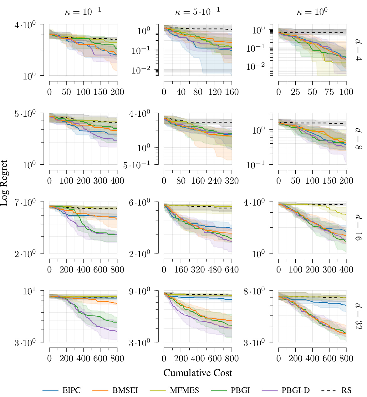
This figure compares the Bayesian regret of different algorithms across various Gaussian process kernels (Matérn 3/2, Matérn 5/2, Squared Exponential) and dimensions (d=4, 8, 16, 32) under uniform costs. The results show that the relative performance of the algorithms varies across different kernels and dimensions, although overall patterns remain consistent. The three distinct performance regimes (easy, medium-hard, very hard) are observed, with the transition points differing based on the kernel and dimension.
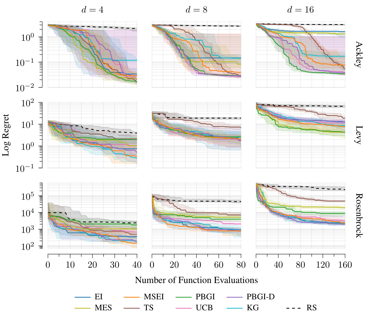
The figure displays the comparison of regret across different synthetic benchmark functions (Ackley, Levy, Rosenbrock) under varying dimensions (d=4, 8, 16). It shows the performance of several Bayesian optimization algorithms (EI, MES, MSEI, TS, PBGI, UCB, PBGI-D, KG) against a random search (RS) baseline. The x-axis represents the number of function evaluations, and the y-axis shows the log regret. The results indicate that for lower dimensions (d=4), most algorithms show similar performance. However, as the dimensionality increases, differences in performance between the algorithms become more pronounced.

This figure compares the performance of several Bayesian optimization algorithms on three different synthetic benchmark functions (Ackley, Levy, and Rosenbrock) across different dimensions (d=4, 8, 16). The results are presented as regret curves, showing the performance of each algorithm in terms of cumulative cost (x-axis) and log regret (y-axis). The dashed black line represents random search (RS) as a baseline. The plot demonstrates that for lower dimensions (d=4), all algorithms exhibit relatively similar performance, but as the dimension increases (d=8, 16), there are noticeable differences in their efficiency and ability to minimize regret, with some algorithms performing considerably better than others.
Full paper#
