↗ OpenReview ↗ NeurIPS Homepage ↗ Chat
TL;DR#
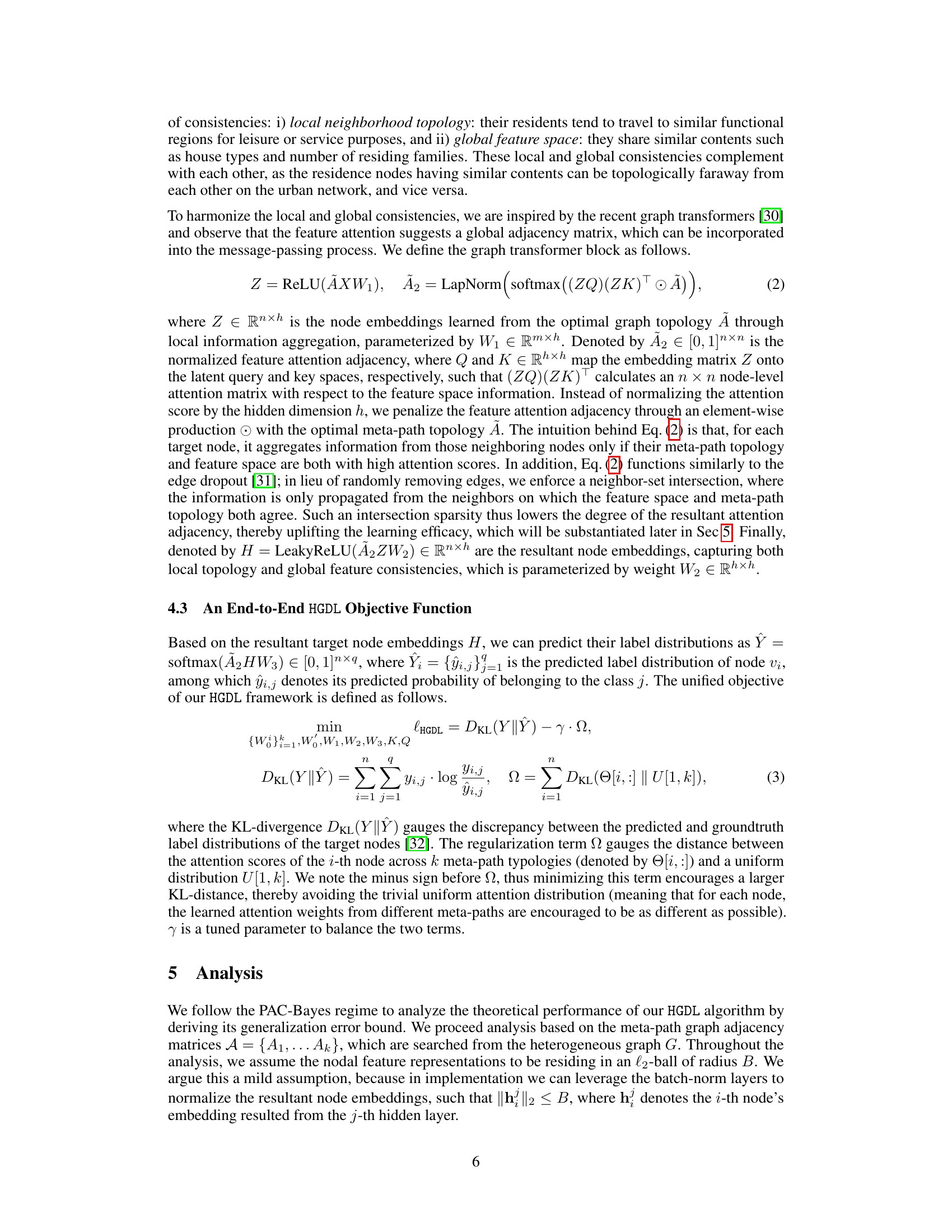
Label Distribution Learning (LDL) traditionally focuses on independent and identically distributed (IID) data. However, real-world data, particularly graph data, often exhibits heterogeneity in node types, attributes, and structures, posing significant challenges for direct application of LDL methods. Existing LDL approaches struggle to effectively handle such heterogeneity, leading to suboptimal label distribution predictions.
This paper introduces Heterogeneous Graph Label Distribution Learning (HGDL), a novel framework designed to address the limitations of existing LDL methods on heterogeneous graphs. HGDL employs a two-component approach: proactive graph topology homogenization to preemptively address node heterogeneity and a topology and content consistency-aware graph transformer to learn consistent representations across meta-paths and node attributes. The proposed framework demonstrates significant performance improvements over existing methods, showcasing its effectiveness in handling the complexities of heterogeneous graph data. The code and datasets are publicly available, facilitating further research and development in the field.
Key Takeaways#
Why does it matter?#
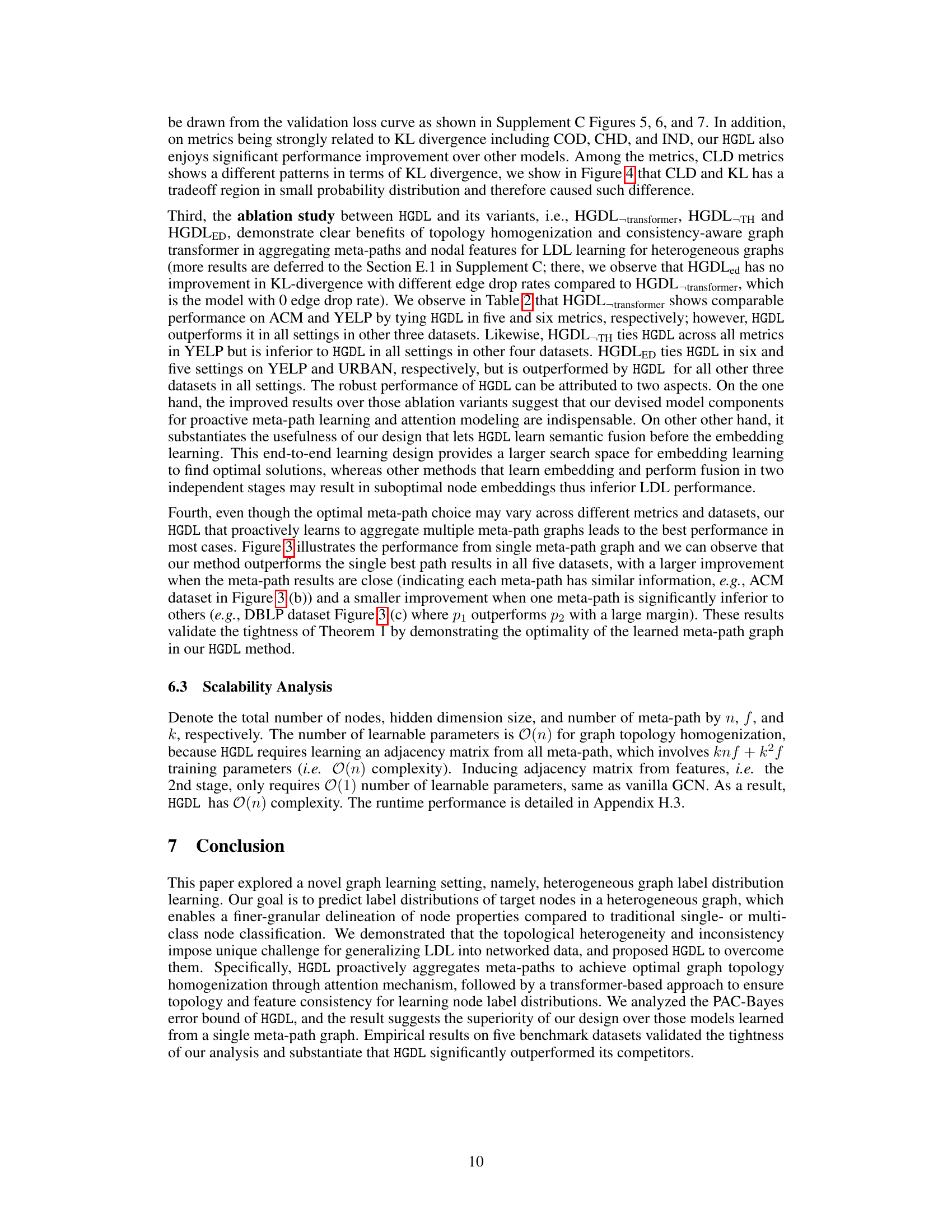
This paper is important because it addresses a critical gap in graph learning research, specifically tackling the challenge of heterogeneous graph label distribution learning. It proposes a novel framework that improves the generalization of label distribution learning in real-world scenarios. This research is relevant to several fields such as urban planning, computer vision, and biomedicine. The proactive topology homogenization and consistency-aware graph transformer are significant advancements in graph learning that pave way for further research and applications.
Visual Insights#
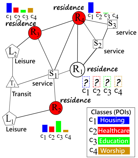
This figure shows an example of a heterogeneous graph representing urban regions. Nodes represent regions with different functionalities (residence, service, leisure, transit), and edges represent taxi services between regions. The goal is to predict the distribution of points of interest (POIs) within each region (represented by the colors in the ‘residence’ nodes), given the region’s type, features, and connections to other regions. The colored nodes show the ground truth label distributions, while uncolored nodes represent those needing prediction.

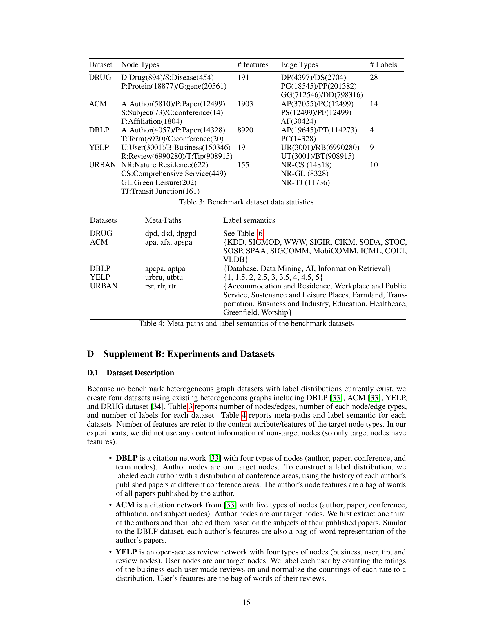
This table summarizes the statistics of five benchmark datasets used in the paper’s experiments. Each dataset is characterized by the number of node types, the total number of nodes, the number of edges, the number of features per node, and the number of labels associated with each node. The datasets represent diverse domains and characteristics, enabling a comprehensive evaluation of the proposed HGDL method.
In-depth insights#
HGDL Framework#
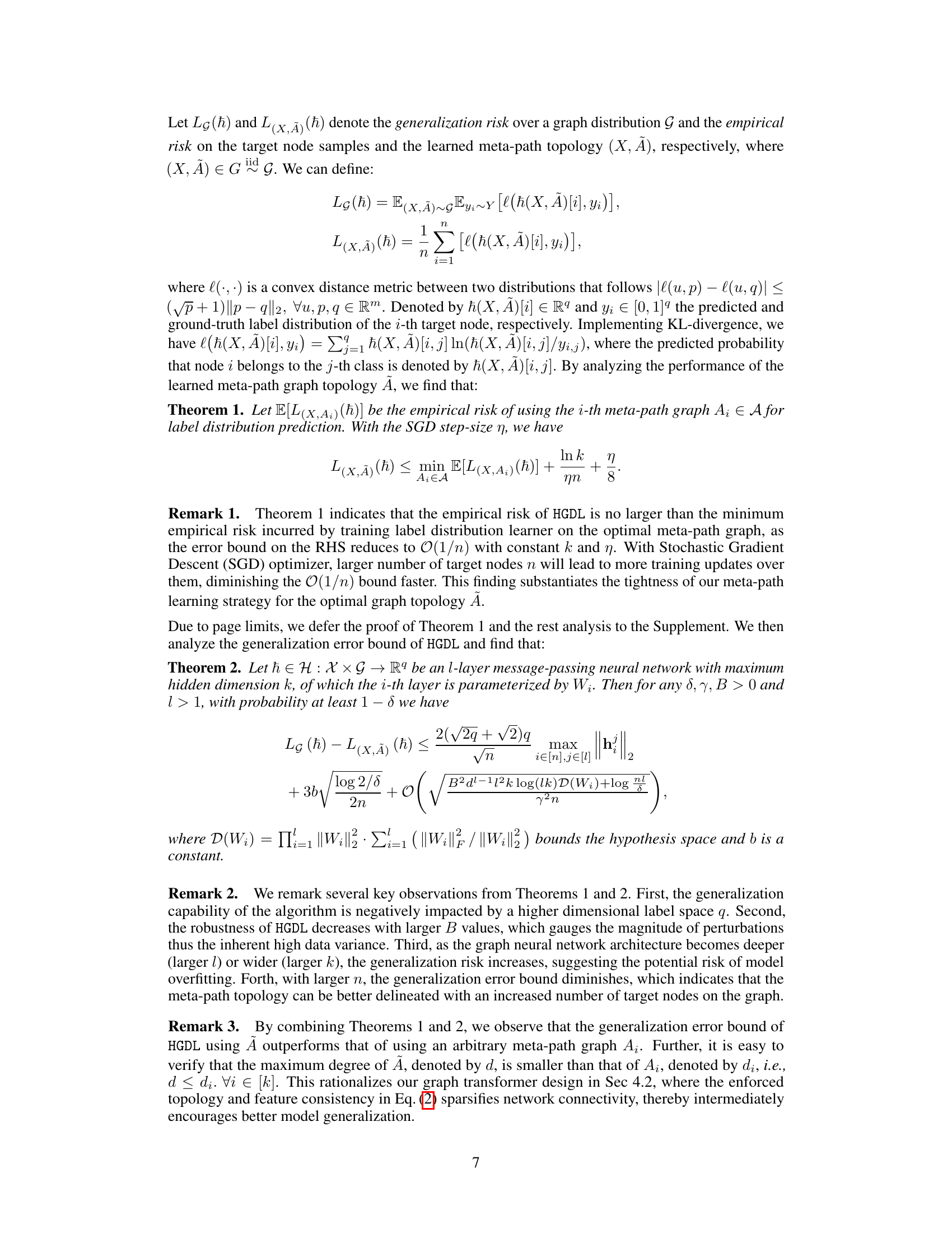
The HGDL framework, proposed for Heterogeneous Graph Label Distribution Learning, is a significant advancement in handling the complexities of real-world graph data. Its core strength lies in its proactive approach, unlike existing methods which reactively aggregate information. HGDL first homogenizes the graph topology using meta-paths and an attention mechanism to address node heterogeneity before proceeding with embedding learning. This proactive step significantly reduces the impact of heterogeneity. Following homogenization, HGDL uses a topology and content consistency-aware graph transformer to combine feature space and topological information, ensuring the embedding process effectively incorporates both aspects. The framework’s end-to-end learning process with a KL-divergence loss function further enhances its efficacy by directly learning label distributions. The theoretical analysis supporting HGDL demonstrates its superiority to existing methods, particularly regarding the generalization error. The experimental results across multiple datasets solidify its effectiveness in real-world scenarios.
Graph Homogenization#
Graph homogenization, in the context of heterogeneous graph label distribution learning, is a crucial preprocessing step to address the challenge of varying node types and structures. The core idea is to transform a heterogeneous graph into multiple homogeneous graphs, each representing a specific meta-path, thereby mitigating the impact of node heterogeneity on subsequent label distribution prediction. This process involves identifying and extracting relevant meta-paths, which are sequences of node types representing different relationships within the graph, to generate simplified graph structures where nodes share similar characteristics. Optimal meta-path selection is key; it aims to capture essential relationships while minimizing redundancy. The resulting homogeneous graphs provide a consistent information propagation pathway, making downstream graph neural network processing more effective. However, simply generating multiple homogenous graphs is insufficient. A mechanism is needed to combine the information from these individual graphs effectively, often through attention mechanisms that weight the importance of each meta-path or graph. This homogenization process is proactive, tackling heterogeneity before embedding learning, leading to more robust and accurate label distribution learning.
Feature-Topology Fusion#
Feature-Topology Fusion is a crucial concept in graph-based machine learning, aiming to integrate the structural information (topology) of a graph with the intrinsic properties (features) of its nodes and edges. Effective fusion is key to unlocking rich representations that capture both local and global contexts. A naive approach might simply concatenate feature vectors with graph embeddings, leading to suboptimal performance. Advanced methods leverage attention mechanisms, graph neural networks, or transformer architectures to learn sophisticated interactions between features and topology. This could involve proactively learning an optimal graph topology that aligns well with the features, or learning mappings that transform features into a topology-aware space. The choice of fusion technique heavily depends on the nature of the data and task, with complex graphs potentially benefiting from techniques that selectively aggregate information from multiple paths before fusing with nodal features. Ultimately, successful feature-topology fusion should yield more accurate and robust predictions by fully leveraging the combined power of graph structure and node content. The quality of the fusion is critical for the overall performance and generalizability of the model.
HGDL Experiments#
The heading ‘HGDL Experiments’ suggests a section detailing the empirical evaluation of the Heterogeneous Graph Label Distribution Learning (HGDL) framework. This section would likely contain a description of the datasets used, chosen for their heterogeneity and representative of real-world scenarios. The experimental setup would be described, including the baselines used for comparison (likely existing graph neural network and LDL methods), evaluation metrics (such as precision, recall, F1-score, and potentially specialized metrics for label distributions), and the experimental procedure itself. Crucially, the results section would present a comparison of HGDL against these baselines, highlighting statistically significant improvements or areas where HGDL might underperform. The analysis may include ablation studies to demonstrate the contribution of each component of the HGDL framework. Overall, the goal is to rigorously validate the claims made about HGDL’s effectiveness in handling heterogeneous graph data and learning accurate label distributions.
HGDL Limitations#
The effectiveness of the Heterogeneous Graph Label Distribution Learning (HGDL) framework, while promising, is subject to certain limitations. Data scarcity remains a significant hurdle, as the creation of heterogeneous graph datasets with ground-truth label distributions is challenging, hindering comprehensive model evaluation. The computational complexity of HGDL scales with the number of nodes (n) and may become computationally expensive with very large graphs. Generalization to unseen data can also be an issue; the performance might not consistently generalize across different datasets exhibiting varying levels of heterogeneity. Although the attention mechanism addresses some heterogeneity, its ability to handle diverse data structures is limited, and parameter tuning is critical for optimal performance but not always straightforward. Finally, the reliance on meta-paths introduces sensitivity towards appropriate choices. Selecting non-optimal meta-paths impacts the accuracy and efficiency of the framework.
More visual insights#
More on figures

This figure illustrates the proposed Heterogeneous Graph Label Distribution Learning (HGDL) framework. It shows the process of converting a heterogeneous graph into multiple homogeneous meta-path graphs, aggregating them using a learnable attention mechanism, and then using a transformer to combine topology and feature information for label distribution prediction. The process is optimized using a joint objective function that balances KL-divergence and an attention regularizer.

This figure compares the performance of the proposed HGDL model against using only a single meta-path for five different datasets. The bar chart displays different evaluation metrics for each method and dataset, offering a visual comparison of their performance. The use of a single meta-path represents a simplified approach compared to HGDL’s more sophisticated method of integrating multiple meta-paths. The results highlight HGDL’s superior performance.
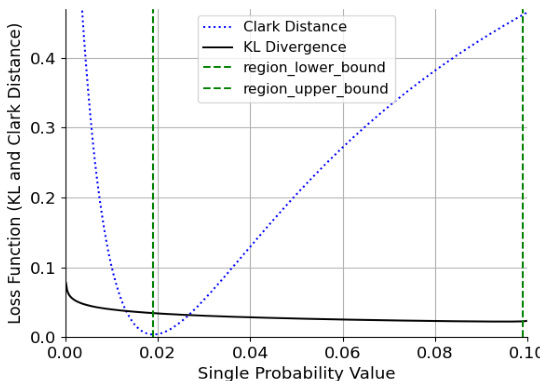
This figure shows an example of the tradeoff between KL divergence and Clark distance. It illustrates how, for a three-class label distribution prediction problem where one class has a high probability (0.9), the KL divergence and Clark distance show an inverse relationship in a certain region. This highlights a limitation of using Clark distance as a metric when one class dominates, as its ability to reflect changes in distribution is limited in these circumstances.

This figure illustrates the proposed Heterogeneous Graph Label Distribution Learning (HGDL) framework. It consists of three main components: 1) Optimal Graph Topology Homogenization, which converts the heterogeneous graph into multiple homogeneous meta-path graphs and learns the optimal topology using an attention mechanism; 2) Topology and Content Consistency-Aware Graph Transformer, which harmonizes the information from the learned optimal topology and nodal features using a transformer architecture; and 3) End-to-End Optimization Objective, which unifies the learning of optimal topology, feature-topology harmonization, and label distribution prediction into a joint optimization problem. This framework aims to effectively address the challenges of heterogeneity and inconsistency in real-world graphs for label distribution learning.

This figure illustrates the HGDL framework, showing how it addresses heterogeneous graph label distribution learning. It starts with a heterogeneous graph and generates multiple homogeneous meta-path graphs. A topology homogenization step learns optimal graph topology through an attention mechanism. A topology and content consistency-aware graph transformer harmonizes nodal features with the learned topology. Finally, a joint optimization objective is used to learn the label distribution for nodes.

This figure compares the performance of HGDL against a baseline model with varying edge drop rates on two datasets: DRUG and ACM. The x-axis represents the edge drop rate, and the y-axis represents the KL loss. The plot shows how the KL loss changes as the edge drop rate increases for both datasets, allowing for a visual comparison of HGDL’s performance relative to the baseline under different levels of edge dropout. This helps illustrate the impact of edge dropout on model performance and the effectiveness of the proposed HGDL approach.
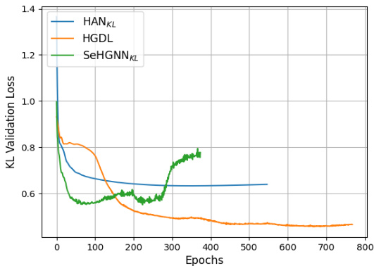
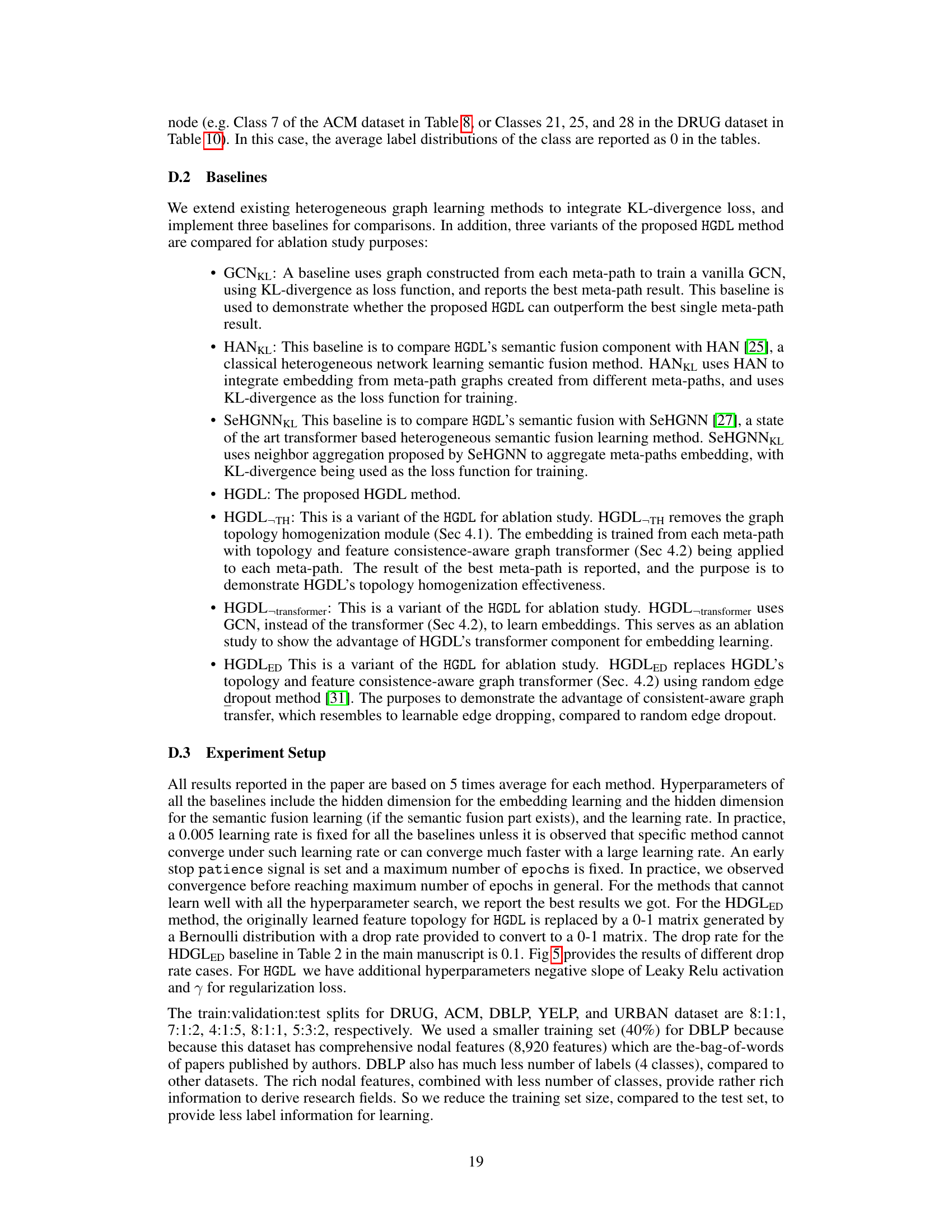
This figure compares the validation KL-divergence loss curves of three different models (HANKL, HGDL, and SeHGNNKL) during training on the ACM dataset. The plot shows how the loss changes over the number of training epochs. Early stopping was used for all three models, so the training ended at different points, but always when no improvement in the loss was observed after a set patience period.

This figure compares the training process KL-divergence validation loss for three different methods (HANKL, HGDL, and SeHGNNKL) on the ACM dataset. It shows how the validation loss changes over epochs. Early stopping is used, meaning training stops when the validation loss stops improving to prevent overfitting. The plot helps illustrate the convergence speed and the final validation loss achieved by each method.
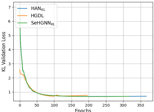
This figure compares the training process KL-divergence validation loss for three different models: HANKL, HGDL, and SeHGNNKL, on the ACM dataset. The plot shows how the validation loss changes over training epochs. Early stopping is used, meaning that training stops when the validation loss stops improving for a certain number of epochs. The figure shows HGDL achieves a lower validation loss compared to the other two models.
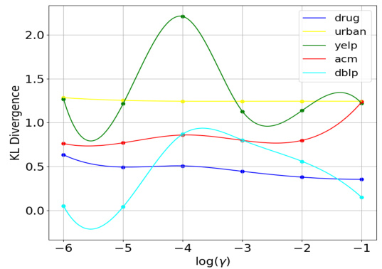
This figure shows the result of a sensitivity analysis performed on the hyperparameter γ. The analysis explores how different values of γ affect the model’s performance, as measured by KL divergence. The x-axis represents the logarithm of γ, while the y-axis shows the KL divergence achieved on five different datasets (DRUG, URBAN, YELP, ACM, DBLP). The figure helps to determine the optimal value of γ for each dataset.
More on tables
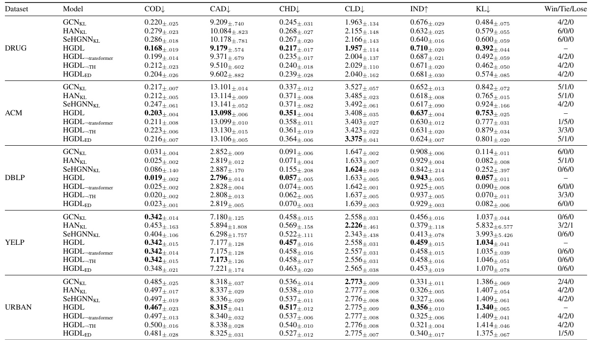
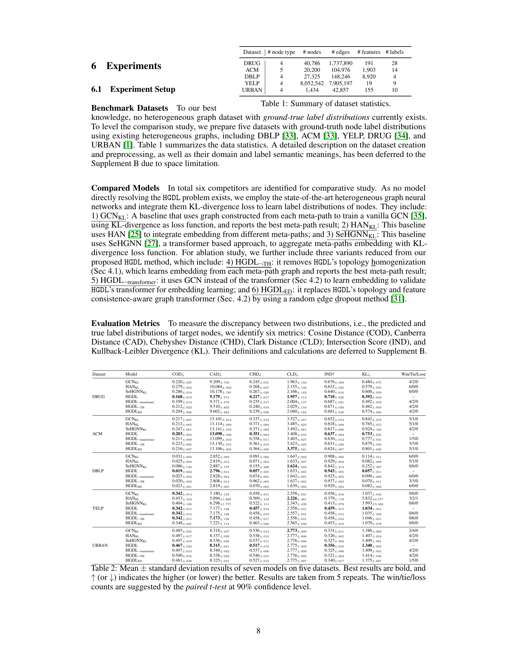
This table presents the performance comparison of seven different models on five graph datasets using six evaluation metrics. The models include baselines and variants of the proposed HGDL model. Each metric measures the discrepancy between predicted and true label distributions. The best-performing model for each metric is highlighted in bold. Win/Tie/Lose counts indicate the number of times each model outperforms, ties, or underperforms HGDL, based on paired t-tests at a 90% confidence level. This provides insights into the effectiveness of HGDL compared to other state-of-the-art methods for heterogeneous graph label distribution learning.

This table presents the statistics of five benchmark datasets used in the paper’s experiments. For each dataset, it lists the number of node types and the count of nodes for each type, the number of features for each node, the edge types and their counts, and the number of labels.

This table summarizes the meta-paths used for each dataset (DRUG, ACM, DBLP, YELP, URBAN) and provides a description of the label semantics for each dataset. Meta-paths represent the different paths through the heterogeneous graph used to generate homogeneous subgraphs for the learning process. The label semantics describe the meaning and interpretation of the labels used in each dataset.

This table shows three examples of drug names, their corresponding Drug IDs, and their chemical structures represented using SMILES notation. SMILES is a simplified way to represent molecular structures as strings, which can be easily processed by computers. This is useful for machine learning models that use molecular information as input.
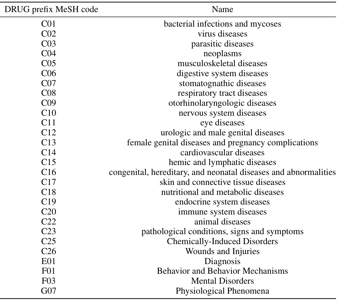
This table shows the semantic meanings of the labels used in the DRUG dataset. Each label represents a category of diseases from the Medical Subject Headings (MeSH) database, which is a comprehensive controlled vocabulary of medical terms. The table provides a mapping between the numerical label identifiers (C01-G07) and the corresponding MeSH categories, clarifying the meaning and nature of the labels used to describe the relationship between drugs and diseases.

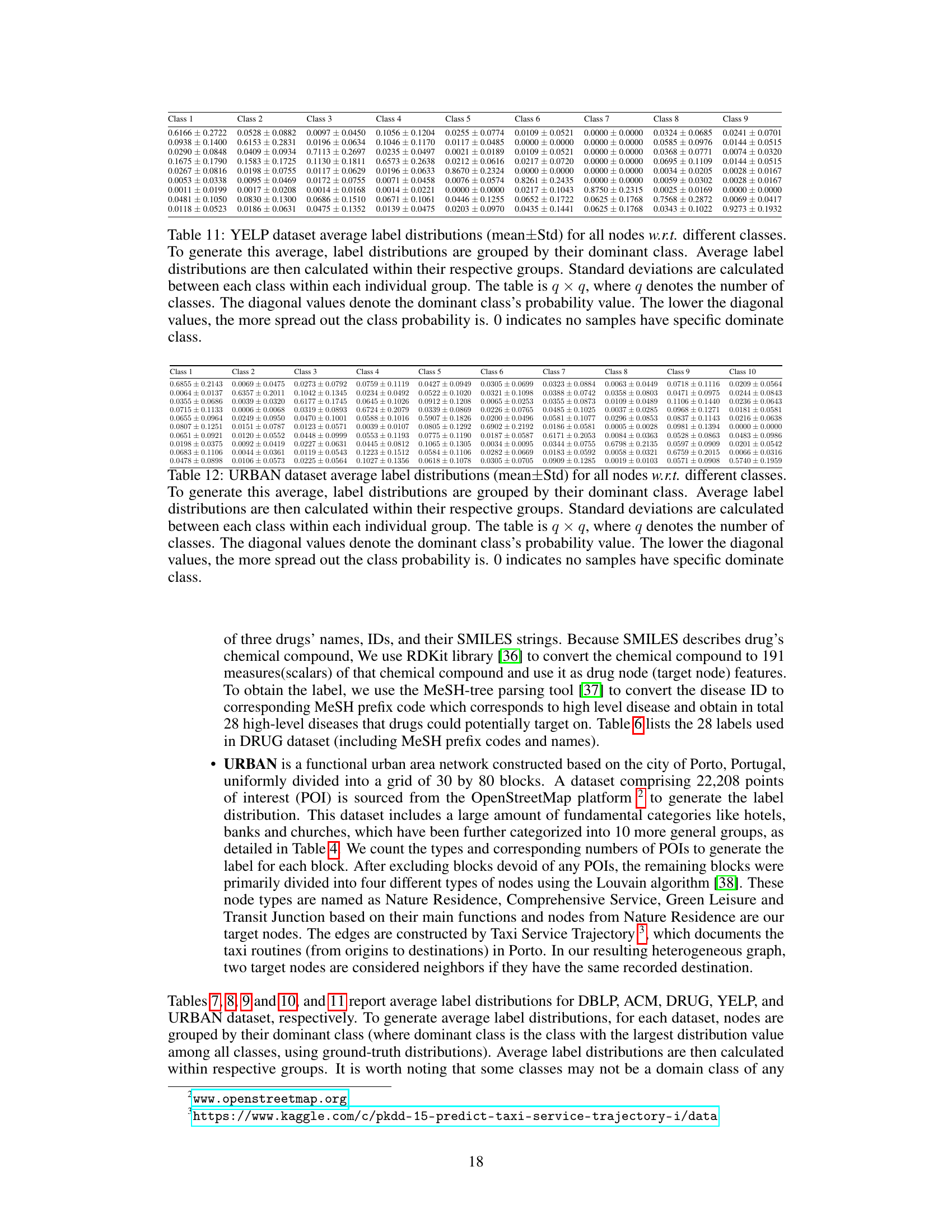
This table shows the average label distributions for each node in the DBLP dataset. Each node’s label is represented as a probability distribution across four classes. The average distribution is calculated by grouping nodes with the same dominant class (the class with the highest probability). Standard deviations show the spread of distributions within each group. Lower diagonal values indicate more spread-out class probabilities.

This table presents the performance comparison of seven models (GCNKL, HANKL, SeHGNNKL, HGDL, HGDL-transformer, HGDL-TH, and HGDLED) across five benchmark datasets (DRUG, ACM, DBLP, YELP, and URBAN). The performance is evaluated using six metrics (COD, CAD, CHD, CLD, IND, and KL) that measure the discrepancy between predicted and true label distributions. The best results for each metric and dataset are highlighted in bold, indicating which model performed best. The win/tie/loss counts show the statistical significance of the differences, obtained through paired t-tests at 90% confidence.

This table presents the performance comparison results of seven models on five different datasets. Each model’s performance is measured using six evaluation metrics: Cosine Distance (COD), Canberra Distance (CAD), Chebyshev Distance (CHD), Clark Distance (CLD), Intersection Score (IND), and Kullback-Leibler Divergence (KL). The best performance for each metric is highlighted in bold. Win/tie/loss counts indicate the number of times each model outperformed, tied, or underperformed the HGDL model across all metrics and datasets.

This table presents the performance comparison of seven different models (including the proposed HGDL model and its variants) on five different datasets. The performance is evaluated using six different metrics: Cosine Distance (COD), Canberra Distance (CAD), Chebyshev Distance (CHD), Clark Distance (CLD), Intersection Score (IND), and Kullback-Leibler Divergence (KL). Lower values are better for COD, CAD, CHD, and CLD, while higher values are better for IND and KL. The win/tie/loss counts represent how many times each model outperformed, tied with, or underperformed the proposed HGDL model at a 90% confidence level based on a paired t-test.
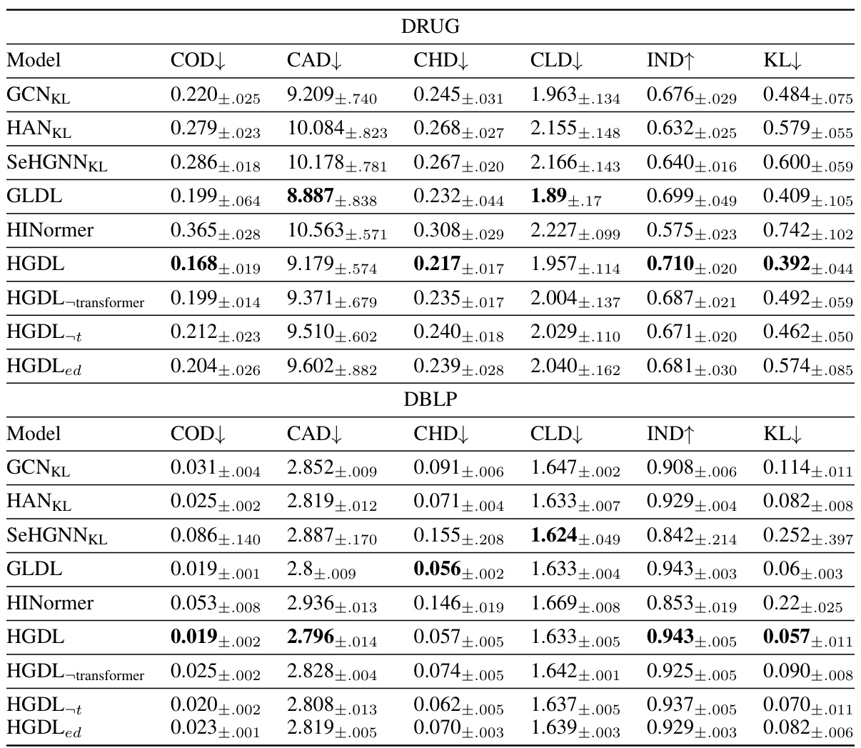
This table presents the performance comparison of seven different models (GCNKL, HANKL, SeHGNNKL, GLDL, HINormer, HGDL, and its variants) on five benchmark datasets (DRUG, ACM, DBLP, YELP, and URBAN) using six evaluation metrics (COD, CAD, CHD, CLD, IND, and KL). The best performance for each metric and dataset is highlighted in bold. The win/tie/loss counts indicate the statistical significance of the performance differences between HGDL and other models.

This table presents the statistics of five benchmark datasets used in the paper. For each dataset, it shows the number of node types, the total number of nodes, the number of edges, the number of features per node, and the number of labels. These datasets cover various domains including biomedicine, scholarly network, business network, and urban planning.
Full paper#
