TL;DR#
Training large neural networks is computationally expensive. One promising solution is to use sparse networks, where many of the connections are removed. However, sparse training is notoriously difficult because removing connections disrupts the flow of information during training, and finding the right settings (hyperparameters) for training is extremely time consuming. These difficulties often lead researchers to re-use the settings that worked for dense networks, even though those settings are often suboptimal.
This paper introduces a new technique called Sparse Maximal Update Parameterization (SµPar) which addresses these issues. SµPar ensures that the flow of information is stable regardless of how sparse the network is, and it uses a clever trick to greatly reduce the time needed for finding optimal hyperparameter settings. Experiments on large language models show that SµPar consistently outperforms existing methods, especially when a high level of sparsity is used. The authors also provide a straightforward implementation, making their work easy for others to adopt and build upon.
Key Takeaways#
Why does it matter?#
This paper is important because it tackles the high computational cost of training large neural networks by addressing the challenges of sparse training. It introduces a novel approach that improves the stability and efficiency of sparse training, enabling researchers to achieve better performance with significantly reduced computational resources. This offers significant implications for hardware acceleration of sparse models and expands the possibilities for training even larger and more complex models.
Visual Insights#
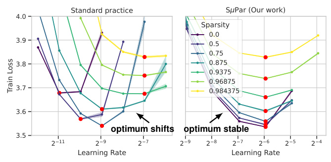
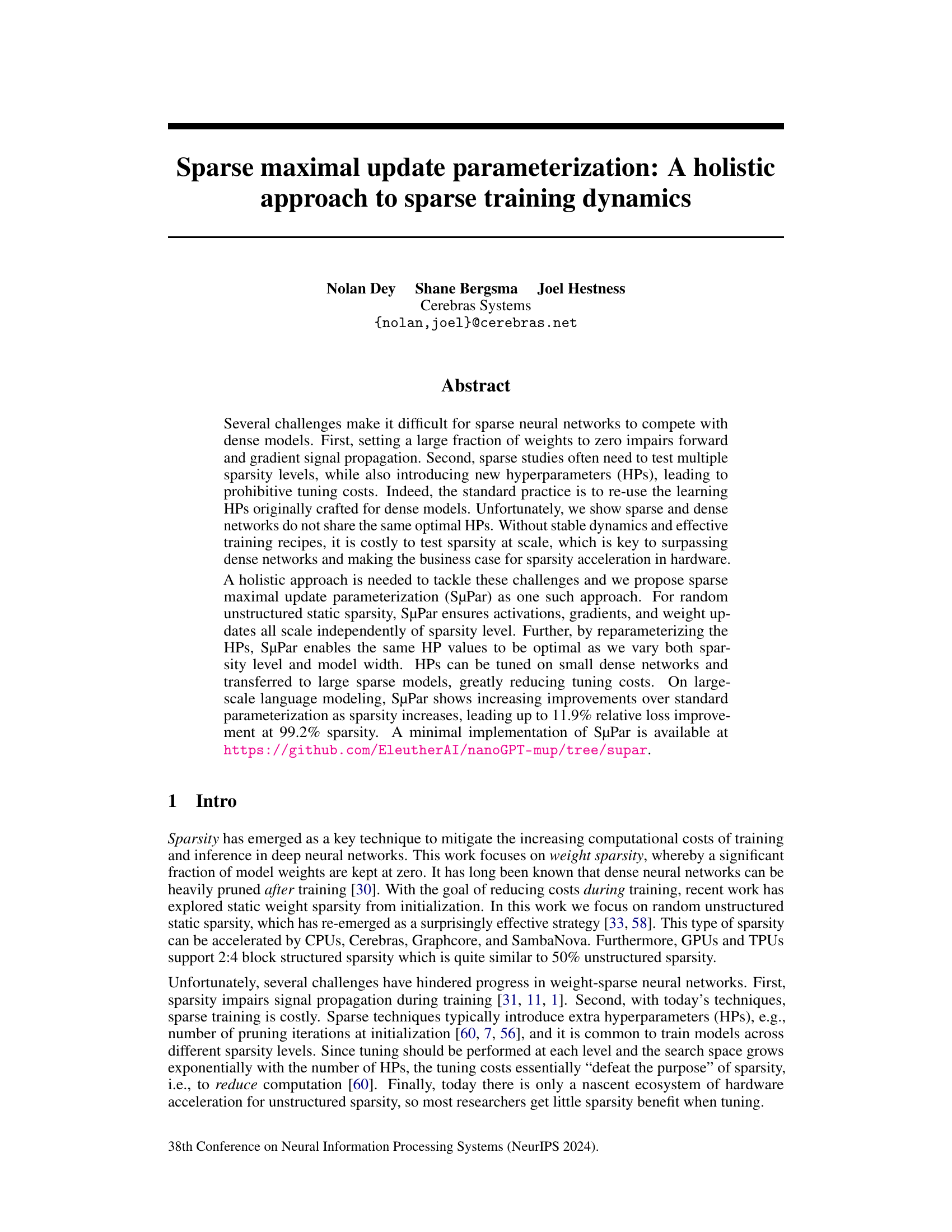
🔼 This figure compares the standard practice of reusing hyperparameters (HPs) optimized for dense models in sparse training versus the SuPar approach. The left panel (Standard Practice) shows that the optimal learning rate shifts significantly as sparsity increases, making it difficult to find good HPs for different levels of sparsity. The right panel (SuPar) demonstrates that SuPar’s reparameterization technique keeps the optimal learning rate stable across all sparsity levels, greatly simplifying hyperparameter tuning for sparse neural networks. This highlights SuPar’s key advantage: enabling efficient and effective training at different sparsity levels without the need for extensive hyperparameter tuning.
read the caption
Figure 1: SuPar (Our work) allows stable optimum HPs for any sparsity level, unlike standard practice.

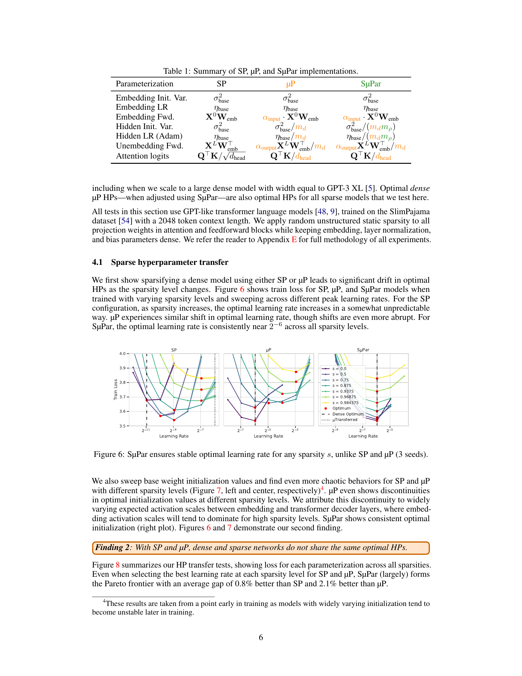
🔼 This table summarizes the differences in the implementations of the Standard Parameterization (SP), Maximal Update Parameterization (µP), and Sparse Maximal Update Parameterization (SµPar) for various parts of a transformer model. It shows how the initialization variance, learning rate, and forward/backward pass calculations differ for embeddings, hidden layers, and attention logits across the three parameterization methods. The table highlights how SµPar incorporates scaling factors related to model width and sparsity to stabilize training dynamics.
read the caption
Table 1: Summary of SP, µP, and SuPar implementations.
In-depth insights#
Sparse Training#
Sparse training techniques aim to reduce the computational cost of training deep neural networks by employing sparsity. Weight sparsity, where a significant portion of network weights are zero, is a common approach. While promising in terms of computational efficiency and memory savings, sparse training faces challenges. Signal propagation issues arise because sparse connections hinder the flow of information during forward and backward passes. Consequently, the training dynamics of sparse models can differ greatly from dense models. Hyperparameter tuning becomes significantly more complex for sparse networks, as the optimal hyperparameters heavily depend on the sparsity level and model architecture. This necessitates exhaustive experiments to find optimal parameters for each sparsity configuration. Effective training recipes for sparse networks remain elusive and are typically not well-established. Therefore, advancements are needed to address the challenges of signal propagation, hyperparameter tuning, and the development of reliable training procedures to harness the full potential of sparse training and overcome its current limitations. Hardware acceleration is another area that needs further development to truly achieve efficiency gains from sparse training.
SuPar Dynamics#
SuPar Dynamics, as a concept, focuses on stabilizing and improving the training dynamics of sparse neural networks. Standard parameterization (SP) and even maximal update parameterization (µP) often struggle with vanishing activations and gradients as sparsity increases. SuPar addresses this by reparameterizing hyperparameters (HPs) such as weight initialization and learning rates to maintain stable activation scales across various sparsity levels and model widths. This enables efficient HP tuning on smaller dense networks, and then transfer the optimal HPs to large sparse models, significantly reducing computational costs. The core of SuPar’s effectiveness lies in its ability to satisfy the Feature Learning Desiderata (FLD), ensuring that activations, gradients, and weight updates remain well-scaled, preventing signal explosion or vanishing and enabling reliable training, even at extremely high sparsity levels. The success of SuPar demonstrates the importance of a holistic approach to sparse training, moving beyond isolated adjustments to address the systemic challenges posed by sparsity.
HP Transfer#
The concept of ‘HP Transfer’ in the context of sparse neural network training is crucial for efficiency. Standard practice often reuses hyperparameters (HPs) optimized for dense models, which is computationally expensive and suboptimal. The core idea behind HP transfer is to leverage HPs tuned on smaller, dense networks and successfully apply them to larger, sparse models. This drastically reduces the cost of hyperparameter optimization, a major bottleneck in sparse training. Successful HP transfer hinges on ensuring the training dynamics of sparse and dense models are sufficiently similar. Therefore, methods that stabilize these dynamics, such as the proposed sparse maximal update parameterization (SµPar), are critical for effective HP transfer. The success of HP transfer demonstrates that carefully designed parameterizations can bridge the gap between dense and sparse training, enabling efficient scaling and broader adoption of sparse neural networks.
Scaling Limits#
Scaling limits in deep learning explore the boundaries of model performance as computational resources increase. Understanding these limits is crucial for predicting future progress and guiding research efforts. Factors affecting scaling include dataset size, model architecture (depth and width), and computational power. While larger models often exhibit improved performance, gains diminish at some point, indicating a limit to scaling’s effectiveness. This could be due to fundamental limitations in model capacity, data sufficiency, or optimization challenges. Research into scaling limits involves analyzing the relationship between model size and performance across various tasks and datasets, revealing the optimal scaling strategies and potentially uncovering architectural improvements that enhance scalability. Furthermore, efficient training methods become paramount at larger scales, prompting investigation into techniques like model parallelism and mixed-precision training. Ultimately, a deep understanding of scaling limits is key to developing more effective and efficient deep learning systems, enabling further advancements in the field.
Future Work#
Future research directions stemming from this work on Sparse Maximal Update Parameterization (SµPar) are plentiful. Extending SµPar to dynamic sparsity methods is crucial, as current formulations assume static sparsity. This necessitates investigating how SµPar’s principles can be adapted to handle evolving sparsity patterns, which may require incorporating techniques from magnitude pruning or other dynamic approaches. Addressing the limitations with non-Gaussian weight distributions is also important. SµPar’s current derivations rely on Gaussian assumptions, therefore research is needed to determine how the parameterization can be generalized for other distributions. Exploring hardware acceleration is another key area, as the computational benefits of sparsity are only fully realized with efficient hardware support. Investigating how SuPar can be optimized for specific hardware architectures is a critical next step to impact real-world applications. Finally, systematic evaluations across diverse architectures and datasets will be valuable. While the paper demonstrates improvements in language modeling, a broader range of model types and tasks would further demonstrate SµPar’s general applicability and robustness.
More visual insights#
More on figures
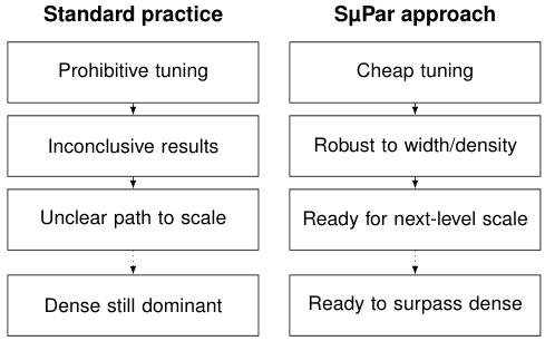
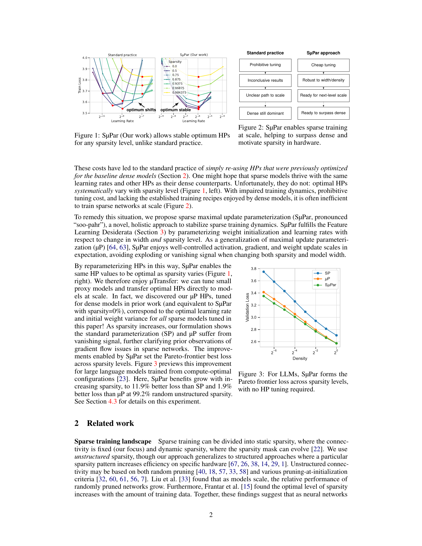
🔼 This figure uses a flowchart to compare the standard practice of sparse training with the SuPar approach. The standard practice is shown to lead to prohibitive tuning costs, inconclusive results, an unclear path to scale, and ultimately, dense models remaining dominant. In contrast, the SuPar approach is depicted as resulting in cheap tuning, results robust to changes in model width and sparsity, a clear path towards scaling to larger models, and ultimately, a potential to surpass dense models.
read the caption
Figure 2: SµPar enables sparse training at scale, helping to surpass dense and motivate sparsity in hardware.
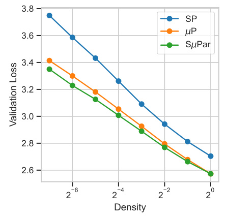
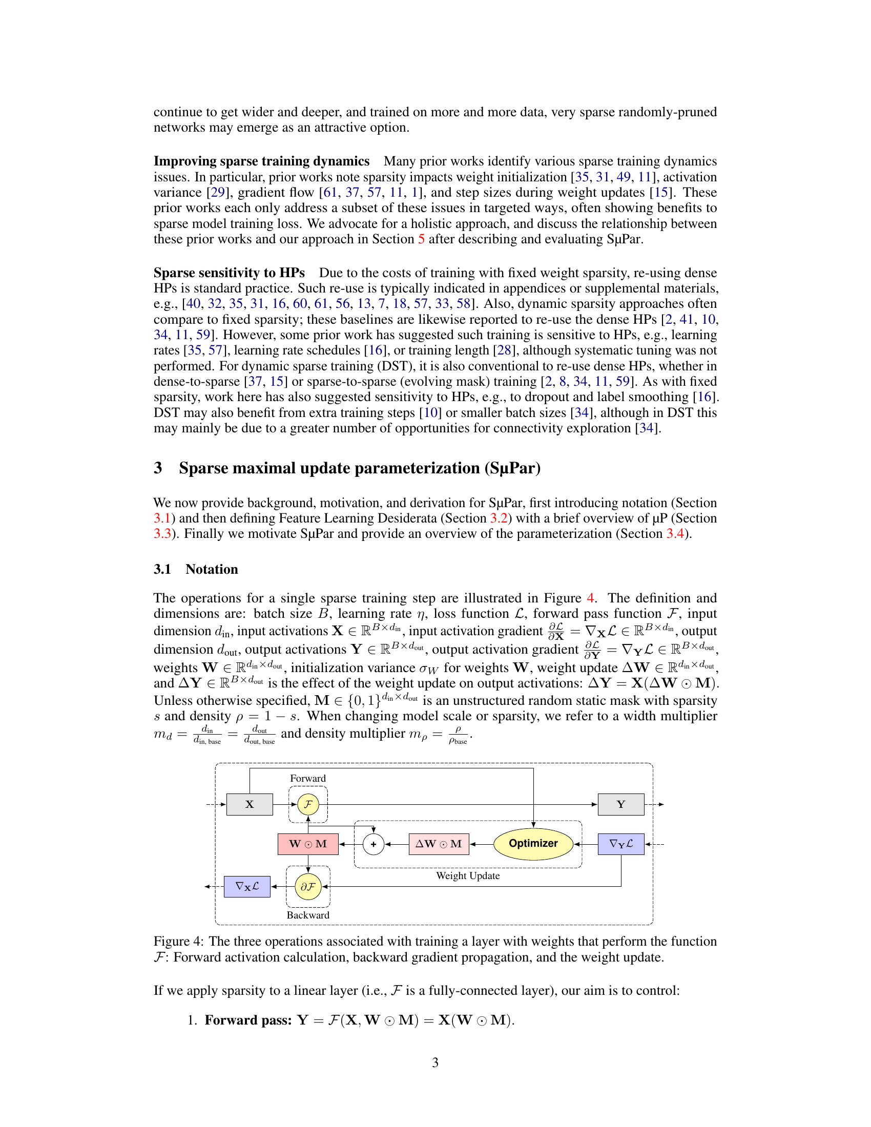
🔼 This figure shows the validation loss of large language models (LLMs) trained with three different parameterizations: standard parameterization (SP), maximal update parameterization (µP), and sparse maximal update parameterization (SµPar). The x-axis represents the density (1 - sparsity) of the model, and the y-axis represents the validation loss. The figure demonstrates that SµPar consistently achieves the lowest validation loss across all sparsity levels, forming the Pareto frontier. This implies that SµPar provides the best trade-off between model sparsity and performance, and requires no hyperparameter tuning across different sparsity levels.
read the caption
Figure 3: For LLMs, SuPar forms the Pareto frontier loss across sparsity levels, with no HP tuning required.
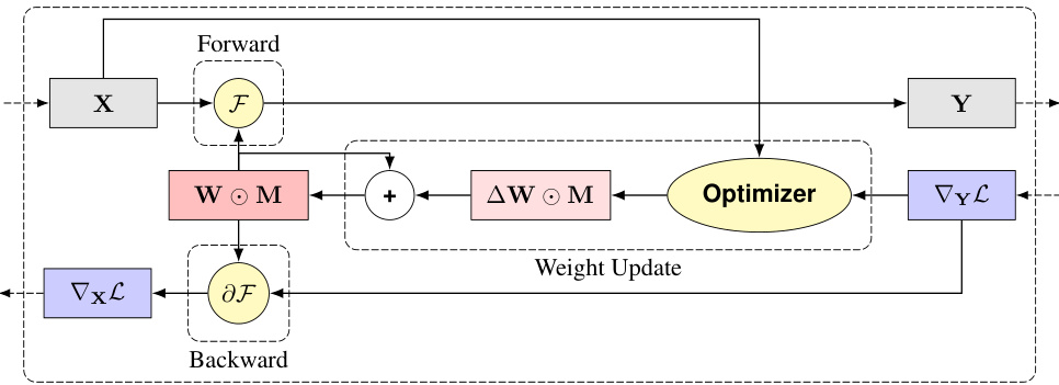
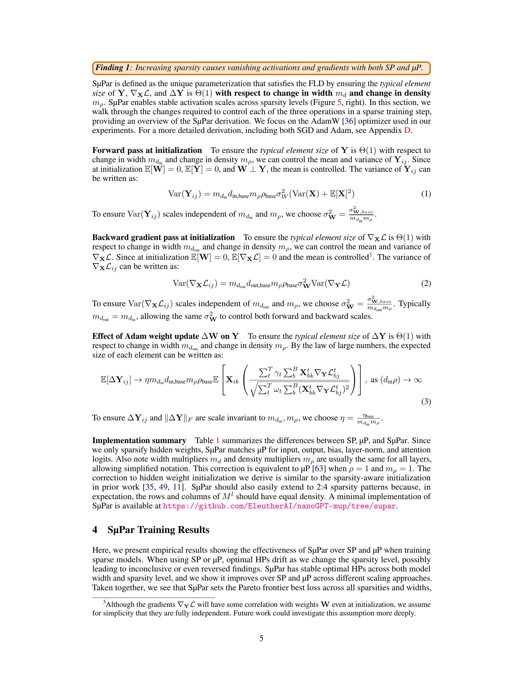
🔼 This figure shows a high-level overview of the three main steps in training a neural network layer using sparse weight updates. The input X is processed by a forward pass function F, which uses a weight matrix W and sparsity mask M. The output of the forward pass is Y. Then, a backward pass calculates the gradient of the loss function with respect to X (∇xL). Finally, an optimizer updates W based on the gradient, incorporating M, resulting in ∆W. This update ∆W is then applied, affecting the next forward pass.
read the caption
Figure 4: The three operations associated with training a layer with weights that perform the function F: Forward activation calculation, backward gradient propagation, and the weight update.
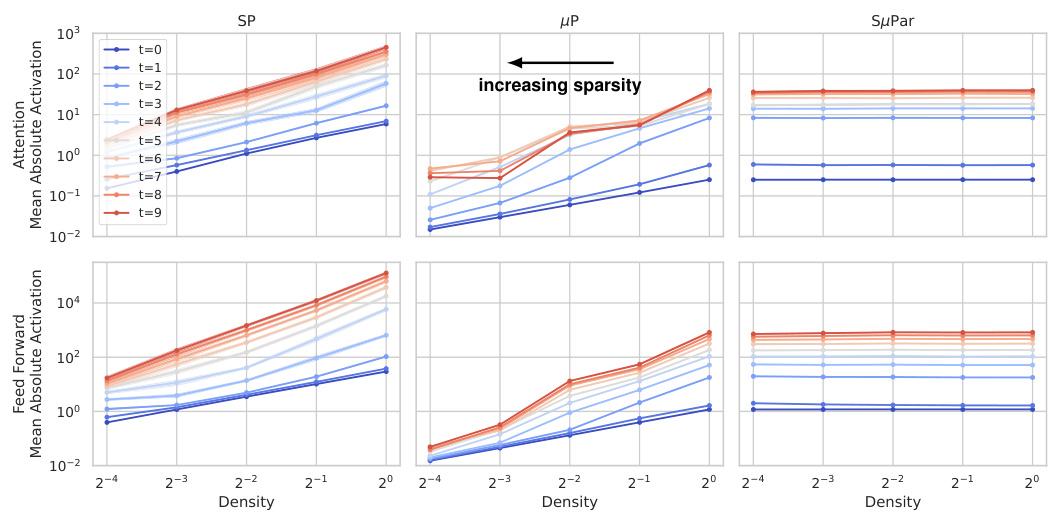
🔼 This figure compares the mean absolute value of activations in attention and feed-forward blocks of a neural network after different training steps for three different parameterization methods: SP (standard parameterization), µP (maximal update parameterization), and SµPar (sparse maximal update parameterization). The x-axis represents the density of the network (1-sparsity), and the y-axis represents the mean absolute activation value. Different lines represent different training steps. The plot shows that with SP and µP, as sparsity increases (density decreases), the activation values tend to vanish. In contrast, with SµPar, the activation values remain relatively stable across different sparsity levels.
read the caption
Figure 5: Mean absolute value activations for attention and feed forward blocks after training step t (10 seeds). In SP and µP models, decreasing density causes activations to vanish (note axes on log-scale). In SµPar models, density has little effect on activation scales and there is no vanishing.

🔼 This figure demonstrates how the optimal learning rate changes with different sparsity levels for three different parameterizations: Standard Parameterization (SP), Maximal Update Parameterization (µP), and Sparse Maximal Update Parameterization (SuPar). For SP and µP, the optimal learning rate shifts significantly as sparsity increases, making it difficult to find a single optimal learning rate that works across all sparsity levels. In contrast, SuPar shows a stable optimal learning rate that remains consistent across various sparsity levels. This highlights SuPar’s ability to stabilize training dynamics and reduce the cost of hyperparameter tuning when training sparse neural networks.
read the caption
Figure 6: SuPar ensures stable optimal learning rate for any sparsity s, unlike SP and µP (3 seeds).

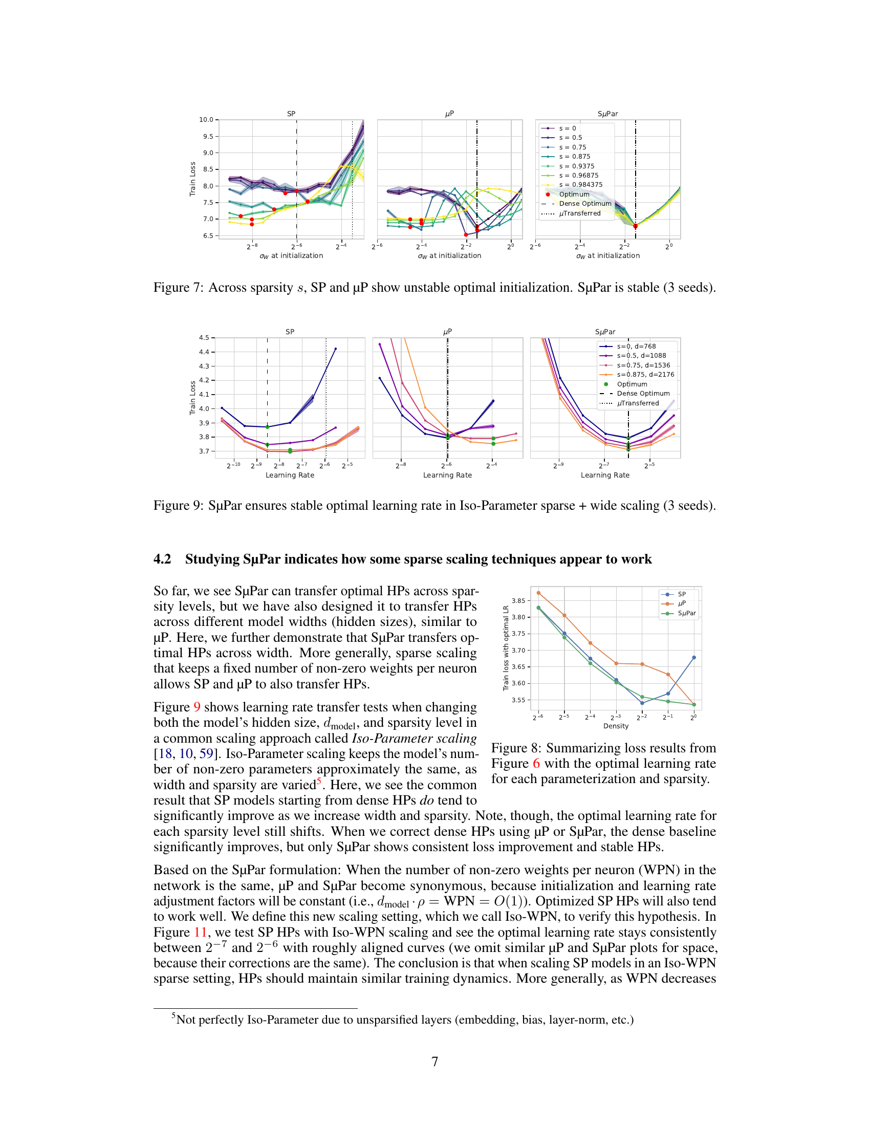
🔼 This figure compares the optimal weight initialization (σw) for different sparsity levels (s) across three different parameterizations: Standard Parameterization (SP), Maximal Update Parameterization (µP), and Sparse Maximal Update Parameterization (SuPar). The x-axis represents the initial weight variance (σw). The y-axis represents the validation loss after training. Each line represents a different sparsity level, ranging from dense (s=0) to highly sparse (s=0.984375). The figure shows that for SP and µP, the optimal σw changes significantly as sparsity increases, demonstrating unstable behavior. In contrast, SuPar maintains a stable optimal σw across all sparsity levels, highlighting its robustness and efficiency in training sparse models.
read the caption
Figure 7: Across sparsity s, SP and µP show unstable optimal initialization. SuPar is stable (3 seeds).

🔼 This figure demonstrates the stability of optimal learning rates across different sparsity levels when using SuPar compared to standard parameterization (SP) and maximal update parameterization (µP). For SP and µP, the optimal learning rate shifts significantly as sparsity increases, whereas SuPar maintains a consistent optimal learning rate near 2⁻⁶ across all sparsity levels. This highlights SuPar’s ability to provide stable training dynamics across varying sparsity levels, which is crucial for efficient sparse training.
read the caption
Figure 6: SµPar ensures stable optimal learning rate for any sparsity s, unlike SP and µP (3 seeds).

🔼 This figure shows the training loss for large language models (LLMs) at different sparsity levels using three different parameterization methods: Standard Parameterization (SP), Maximal Update Parameterization (µP), and Sparse Maximal Update Parameterization (SµPar). The x-axis represents the model density (1-sparsity), while the y-axis shows the validation loss. The figure demonstrates that SuPar consistently achieves the lowest training loss across all sparsity levels, forming the Pareto frontier – meaning there is no other parameterization that achieves better loss at any given sparsity. Importantly, SuPar achieves this without requiring any hyperparameter tuning across different sparsity levels; the optimal hyperparameters remain stable.
read the caption
Figure 3: For LLMs, SuPar forms the Pareto frontier loss across sparsity levels, with no HP tuning required.
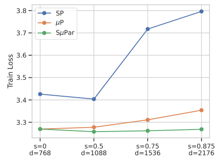
🔼 This figure demonstrates the stability of optimal learning rates across various sparsity levels when using SuPar (sparse maximal update parameterization). It contrasts SuPar’s performance with standard parameterization (SP) and maximal update parameterization (µP). SuPar shows consistent optimal learning rates across different sparsity levels, unlike SP and µP, which exhibit significant drift in optimal learning rates as sparsity increases. This highlights SuPar’s ability to maintain stable training dynamics across various sparsity levels, simplifying hyperparameter tuning and improving the efficiency of sparse training.
read the caption
Figure 9: SuPar ensures stable optimal learning rate for any sparsity s, unlike SP and µP (3 seeds).
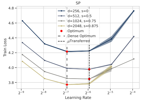
🔼 This figure demonstrates the stability of optimal learning rates across various sparsity levels using the SuPar approach, in contrast to the standard parameterization (SP) and maximal update parameterization (µP). The graph shows training loss plotted against learning rate for different sparsity levels (s). SuPar maintains a consistent optimal learning rate across all sparsity levels, whereas SP and µP show significant shifts in the optimal learning rate as sparsity increases. This highlights SuPar’s ability to stabilize optimal hyperparameters, which is crucial for efficient and effective sparse training.
read the caption
Figure 6: SµPar ensures stable optimal learning rate for any sparsity s, unlike SP and µP (3 seeds).
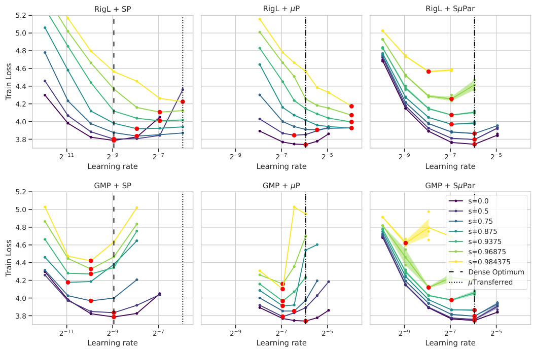
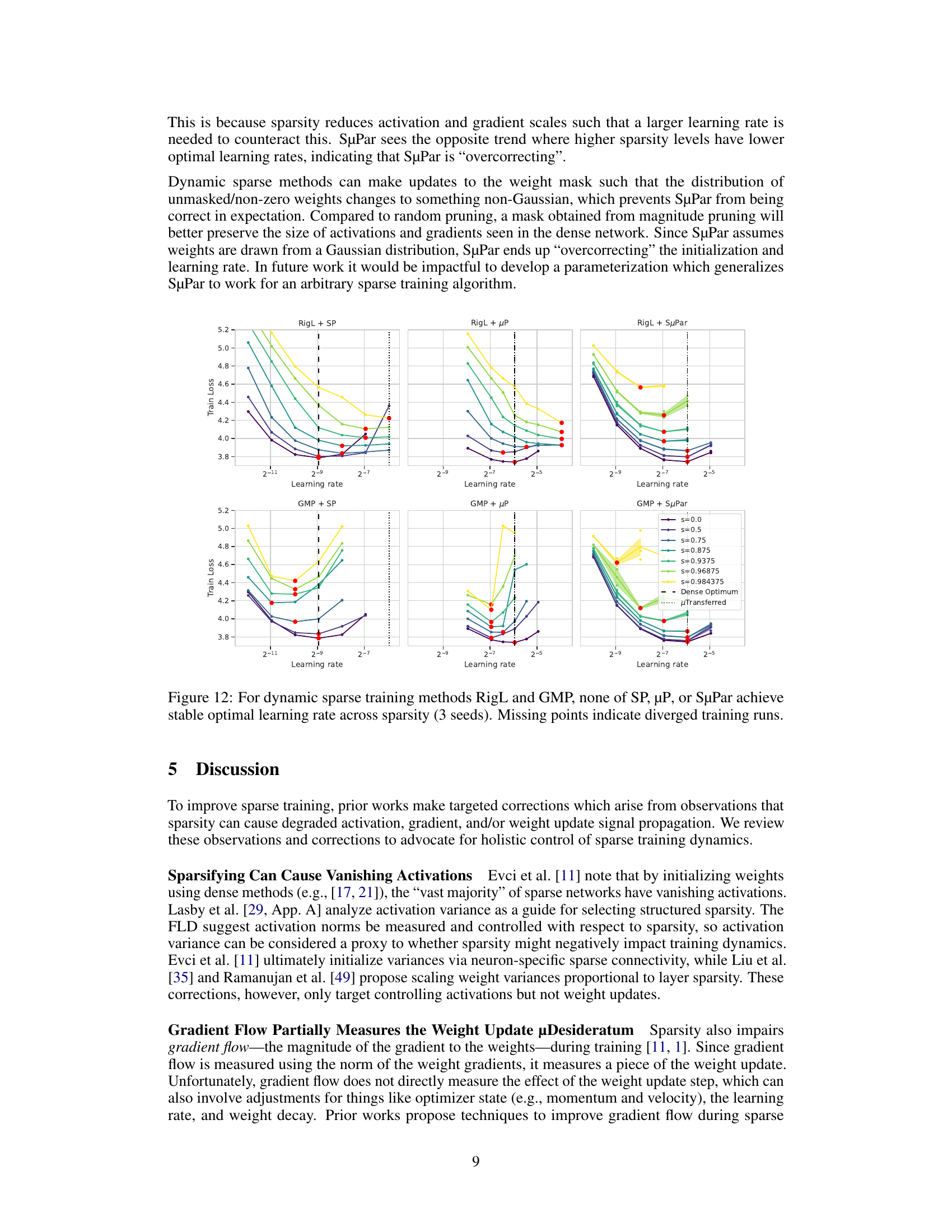
🔼 This figure demonstrates the instability of optimal learning rates across different sparsity levels for various dynamic sparse training methods (RigL and GMP) when combined with standard parameterization (SP), maximal update parameterization (µP), and sparse maximal update parameterization (SµPar). The instability is highlighted by the scattered optimal learning rate values across sparsity levels for all three parameterization methods, indicating that a single optimal learning rate does not exist across varying sparsity for these methods. The missing data points for several configurations suggest the training process diverged for certain hyperparameter settings and sparsity levels.
read the caption
Figure 12: For dynamic sparse training methods RigL and GMP, none of SP, µP, or SuPar achieve stable optimal learning rate across sparsity (3 seeds). Missing points indicate diverged training runs.

🔼 This figure compares the weight initialization standard deviation across different sparsity levels for four different parameterizations: SP, μP, μP + SuPar init only (using SuPar initialization but μP learning rate), and μP + SµPar LR only (using SuPar learning rate but μP initialization). The x-axis represents σw at initialization, and the y-axis represents training loss. The plot demonstrates that only SuPar achieves stable optimal weight initialization standard deviation across all sparsity levels.
read the caption
Figure 13: SµPar ensures stable optimal weight initialization standard deviation, unlike SP, μP, μP + SuPar init only, and μP + SµPar LR only.

🔼 This figure compares the performance of different parameterization methods (SP, µP, µP + SuPar init only, µP + SuPar LR only, and SuPar) across various sparsity levels. Each line represents a different sparsity level, and the red dot on each line indicates the optimal learning rate for that sparsity level. The figure demonstrates that SuPar achieves a stable optimal learning rate across all sparsity levels, unlike the other methods, where the optimal learning rate shifts significantly as sparsity changes. This highlights SuPar’s ability to maintain stable training dynamics despite varying sparsity.
read the caption
Figure 14: SµPar ensures stable optimal learning rate (Bottom), unlike SP, µP, µP + SµPar init only, and µP + SµPar LR only.
More on tables
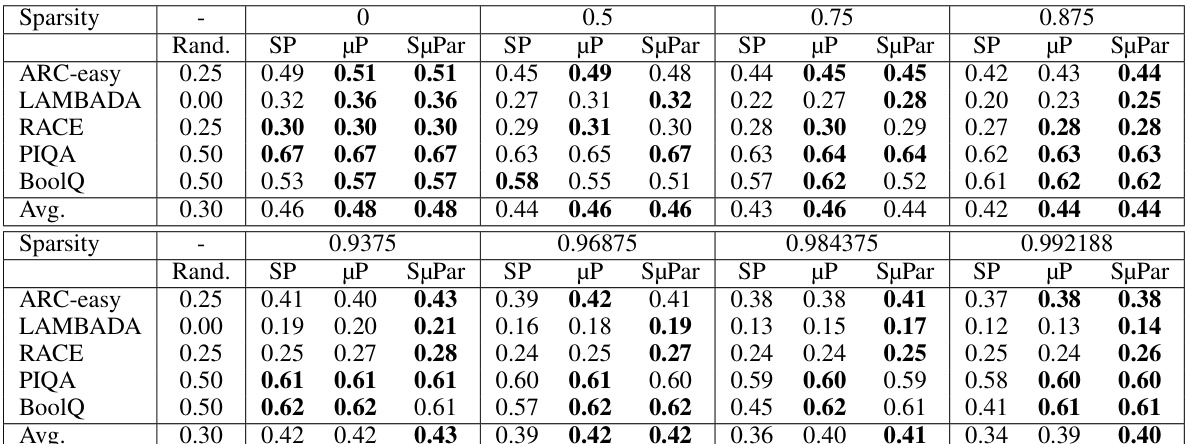
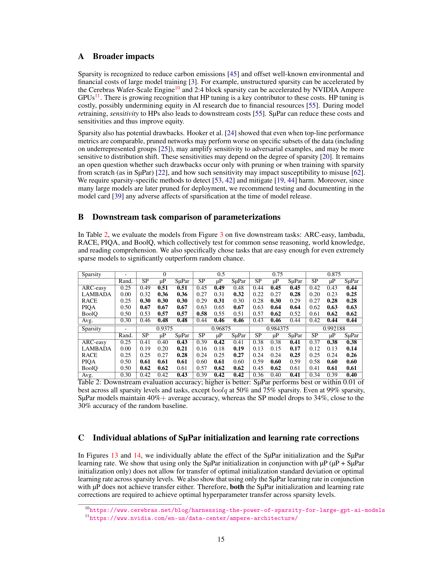
🔼 This table presents the results of evaluating several language models on five downstream tasks (ARC-easy, LAMBADA, RACE, PIQA, and BoolQ) with varying levels of sparsity (0%, 50%, 75%, 87.5%, 93.75%, 96.875%, 98.4375%, and 99.2188%). The models were trained using three different parameterization methods: standard parameterization (SP), maximal update parameterization (µP), and sparse maximal update parameterization (SµPar). The table shows the average accuracy across the five downstream tasks for each sparsity level and parameterization method. It highlights that SµPar consistently outperforms SP and µP, particularly at higher sparsity levels, demonstrating its effectiveness in maintaining high accuracy even with significant sparsity.
read the caption
Table 2: Downstream evaluation accuracy; higher is better: SµPar performs best or within 0.01 of best across all sparsity levels and tasks, except boolq at 50% and 75% sparsity. Even at 99% sparsity, SuPar models maintain 40%+ average accuracy, whereas the SP model drops to 34%, close to the 30% accuracy of the random baseline.
🔼 This table summarizes the differences in how the standard parameterization (SP), maximal update parameterization (µP), and sparse maximal update parameterization (SµPar) approaches handle various hyperparameters during training, focusing on weight initialization variance, learning rates, and forward weight transformations for embedding and hidden layers. The table highlights the key distinctions in how each method scales these parameters with respect to changes in model width and sparsity.
read the caption
Table 1: Summary of SP, µP, and SuPar implementations.

🔼 This table summarizes the differences in implementation between the standard parameterization (SP), maximal update parameterization (µP), and the proposed sparse maximal update parameterization (SµPar). It shows how the initialization variance, learning rate, and forward pass calculations differ for embeddings, hidden layers, and attention logits across the three methods, highlighting the key differences in how each approach handles the scaling of activations, gradients, and weights with respect to changes in model width and sparsity.
read the caption
Table 1: Summary of SP, µP, and SuPar implementations.
Full paper#
