TL;DR#
Decoding natural images from brain activity is a challenging but crucial task in neuroscience. Current methods often struggle to reconstruct complex visual scenes accurately and lack the ability to resolve the temporal dynamics of neural activity. This limits our understanding of how the brain represents and processes visual information. This research aims to improve the accuracy and resolution of image reconstruction from neural signals, and to gain deeper insights into brain mechanisms.
The MonkeySee project uses a convolutional neural network (CNN) to decode naturalistic images from multi-unit activity (MUA) recordings in macaque brains. The method includes a novel space-time-resolved decoding technique and an interpretable layer that maps brain signals to 2D images dynamically. This allows for high-precision image reconstructions and helps understand how the brain’s representations translate into pixels. The results demonstrate high-fidelity reconstructions of naturalistic images and reveal distinct readout characteristics for neuronal populations from different brain areas (V1, V4, and IT). This research pushes the boundaries of current neural decoding techniques and deepens our understanding of how the brain processes visual information.
Key Takeaways#
Why does it matter?#
This paper is important because it significantly advances our understanding of how the brain processes visual information by introducing novel space-time resolved decoding techniques and highly accurate image reconstruction from brain signals. It opens new avenues for research in neuroprosthetics and brain-computer interfaces by demonstrating the feasibility of reconstructing natural images from neural activity, paving the way for more realistic and effective visual prostheses. Furthermore, the use of a learned receptive field layer provides insights into how CNN models internally process information, which has implications for improving the accuracy and interpretability of future neural decoding models. The innovative methods introduced, like the end-to-end inverse retinotopic mapping, can be adopted in other neuroscience research involving neural decoding.
Visual Insights#

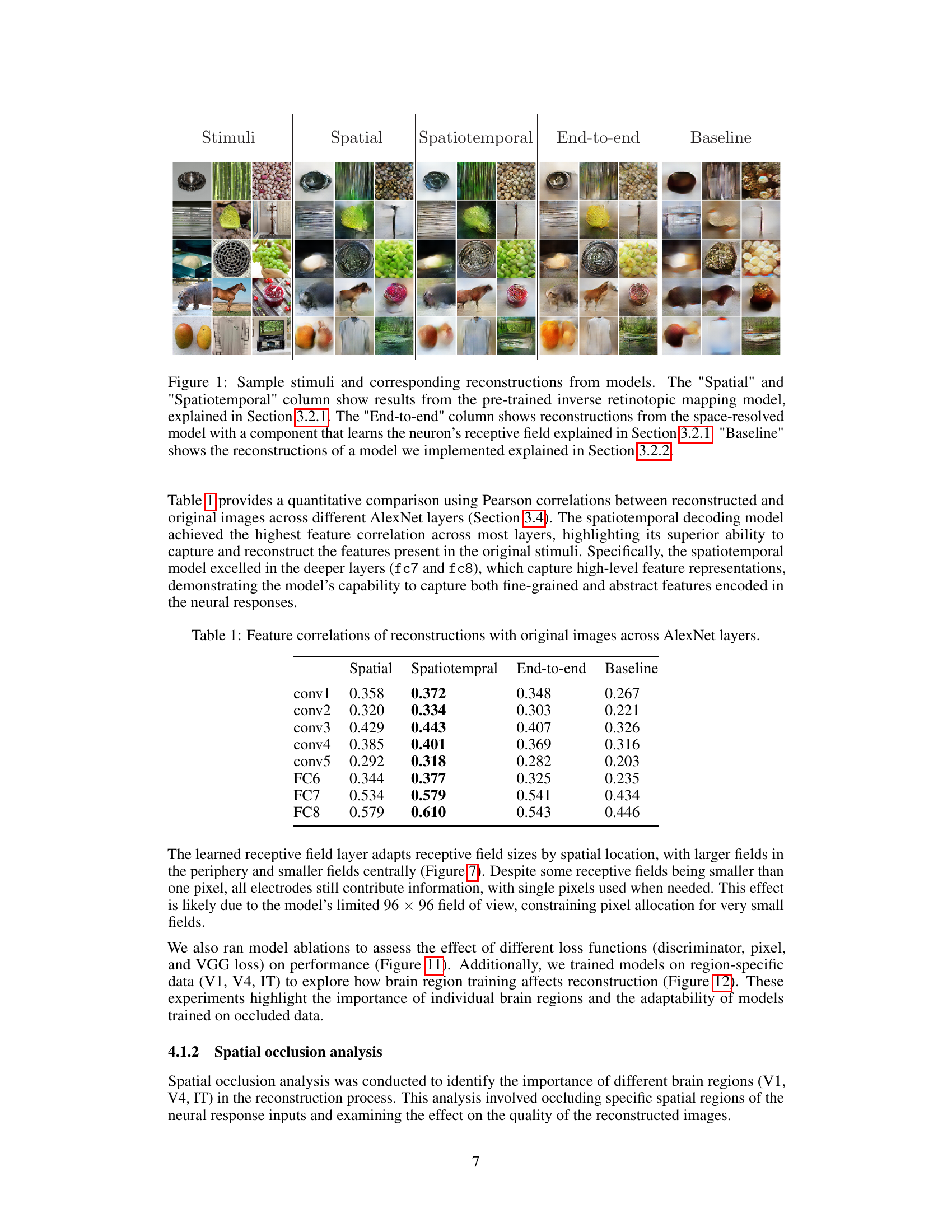
🔼 This figure shows a comparison of image reconstruction results from four different decoding models: a spatial model, a spatiotemporal model, an end-to-end model, and a baseline model. Each model’s performance is evaluated on a set of sample images. The results illustrate the models’ abilities to reconstruct various image features, and highlights the improvements achieved by incorporating spatiotemporal information and a learned receptive field layer.
read the caption
Figure 1: Sample stimuli and corresponding reconstructions from models. The 'Spatial' and 'Spatiotemporal' column show results from the pre-trained inverse retinotopic mapping model, explained in Section 3.2.1. The 'End-to-end' column shows reconstructions from the space-resolved model with a component that learns the neuron's receptive field explained in Section 3.2.1. 'Baseline' shows the reconstructions of a model we implemented explained in Section 3.2.2.
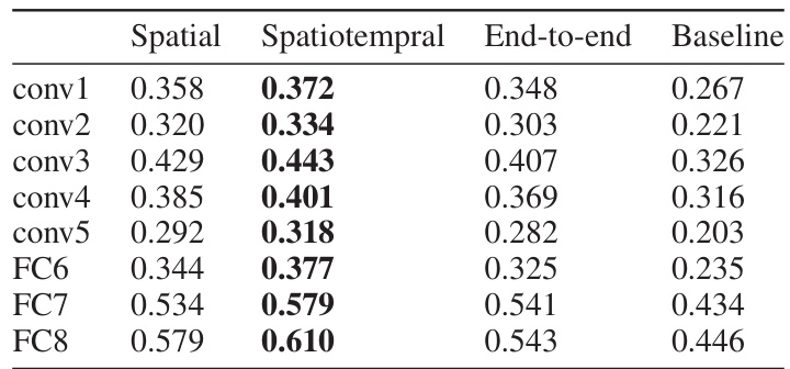
🔼 This table presents a quantitative comparison of the reconstruction performance of different decoding models (spatial, spatiotemporal, end-to-end, and baseline) using Pearson correlations between reconstructed and original images across various layers of a pre-trained AlexNet. Higher correlation values indicate better reconstruction of the image features present in the original image. The table helps to assess the relative effectiveness of each model at capturing various levels of visual information.
read the caption
Table 1: Feature correlations of reconstructions with original images across AlexNet layers.
In-depth insights#
CNN Decoding#
CNN decoding, in the context of neuroscience, uses convolutional neural networks (CNNs) to reconstruct sensory information directly from brain activity. This technique is particularly powerful when dealing with complex, naturalistic stimuli like images and videos, as CNNs are adept at capturing spatial hierarchies of features. The process often involves training a CNN as a decoder, mapping brain activation patterns to pixel values. Effective decoding often necessitates large, diverse datasets of brain recordings paired with the corresponding stimuli to ensure the model learns robust and generalizable mappings. The success of CNN decoding hinges on the model’s capacity to learn and disentangle complex, high-dimensional relationships between neural responses and the sensory world. Furthermore, the interpretability of the CNN decoding model is critical. Understanding how the model’s internal representations translate into decoded features offers valuable insights into the nature of cortical computations and provides a window into the brain’s internal representations. The application of this methodology is advancing our understanding of visual processing, especially in relation to high-level visual areas of the brain and how they process complex naturalistic scenes.
Retinotopic Mapping#
Retinotopic mapping is a crucial concept in visual neuroscience, referring to the spatial organization of the visual field onto the visual cortex. The paper investigates how this spatial arrangement is encoded in neural activity and subsequently decoded to reconstruct natural images. A key aspect is understanding how different brain regions (V1, V4, and IT) contribute to the retinotopic map and the characteristics of their neural representations. The authors introduce a novel method using convolutional neural networks (CNNs) to achieve this, focusing on the efficiency and interpretive capacity of the model. The integration of a learned receptive field layer enhances model performance and further elucidates how the brain translates neural activity patterns into visual images. The space-time resolved approach allows investigation of the temporal dynamics of retinotopic mapping, improving our understanding of visual processing. The homeomorphic decoder, a fully convolutional model, highlights the importance of spatial and temporal neural signals for high-fidelity image reconstruction. Therefore, the study uses retinotopic mapping as a powerful tool to explore the brain’s representations of visual information and how neural decoding can be optimized using CNN based decoders. This research promises to significantly advance our understanding of visual perception.
Temporal Dynamics#
The temporal dynamics of neural processing are crucial for understanding visual perception. The study’s innovative space-time resolved decoding technique directly addresses this by analyzing neuronal signals across specific time intervals aligned with known latency periods in the visual pathway (V1 to IT). This approach moves beyond static image reconstruction, providing insights into how visual information unfolds over time. By incorporating these temporal dynamics, the model offers a more complete and accurate understanding of neural representations. The results demonstrate how temporal resolution enhances the fidelity of visual reconstructions and further our understanding of the brain’s complex processing mechanisms. This temporal aspect is a significant contribution, going beyond typical decoding methods which focus mainly on spatial relationships.
Model Inference#
Model inference in the context of decoding naturalistic images from neural activity involves investigating how a neural network model interprets and reconstructs visual stimuli from brain signals. A crucial aspect is understanding how the network processes spatially separated brain regions. The authors likely employed techniques like truncated brain data input or selective masking of regions to analyze the model’s response. This would reveal how the model integrates information from different brain areas and the hierarchical nature of visual processing. Results might show distinct contributions from regions like V1, V4, and IT, highlighting the efficiency of the model’s organization and how well it replicates known neurobiological pathways. Furthermore, investigating model inference is critical for determining the model’s interpretability and enhancing our understanding of brain representations. Analysis may involve probing the model’s internal layers or activations, potentially relating them to specific visual features or spatial locations in the reconstructed image. The goal is to demonstrate the model’s ability to learn meaningful relationships between neural activity and visual features, and how this relationship unfolds across the brain’s visual hierarchy. Analyzing the model’s inference in this way is vital for validating its capacity to accurately reflect neurobiological processes and its potential for practical applications like neuroprosthetics.
Occlusion Effects#
Occlusion studies in visual neuroscience aim to understand how the brain processes visual information when parts of the scene are hidden. By systematically masking or removing parts of the stimulus, researchers can identify the critical visual features necessary for accurate object recognition and scene reconstruction. The results often demonstrate a hierarchical processing of visual information; low-level areas focus on local features, while higher-level areas integrate more global information. Occlusion analyses can reveal which brain regions are most sensitive to specific visual features and at what stage of processing these sensitivities appear. For example, occluding parts of an image might reveal whether object recognition relies heavily on local texture or global shape. In the context of deep learning models, occlusion experiments can provide insight into how the model’s representations mirror those of the brain, allowing for a comparison of performance and a better understanding of both biological and artificial systems. Such comparative analyses are crucial for evaluating the validity of computational models and refining them to better reflect biological mechanisms. Moreover, the use of neural recordings, combined with occlusion experiments, could inform the design of more robust and effective visual neuroprosthetics by identifying the crucial information that needs to be accurately restored to achieve functional vision.
More visual insights#
More on figures
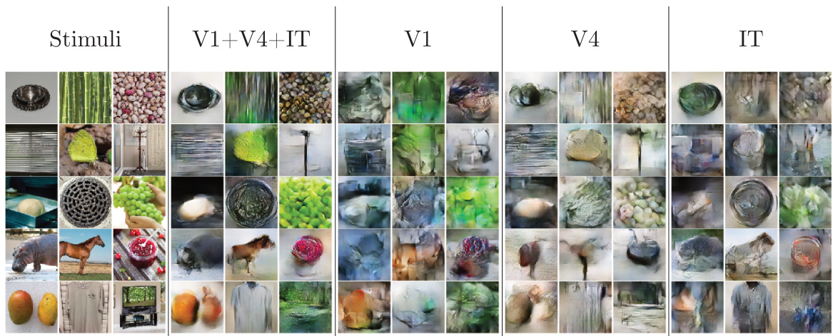
🔼 This figure shows the results of a spatial occlusion analysis, where the model’s input from different brain regions (V1, V4, IT) was selectively occluded. The columns represent the regions of interest, while the rows present different example stimuli. For each region, the neural responses were set to their baseline values (pre-stimulus onset) for the occlusion procedure. The reconstructions demonstrate how the absence of input from a specific brain area impacts the final reconstructed images, highlighting the importance of each brain area’s contribution to visual processing.
read the caption
Figure 2: Spatial occlusion analysis of spatial model as explained in Section 4.1.2. Title above column means included brain region.

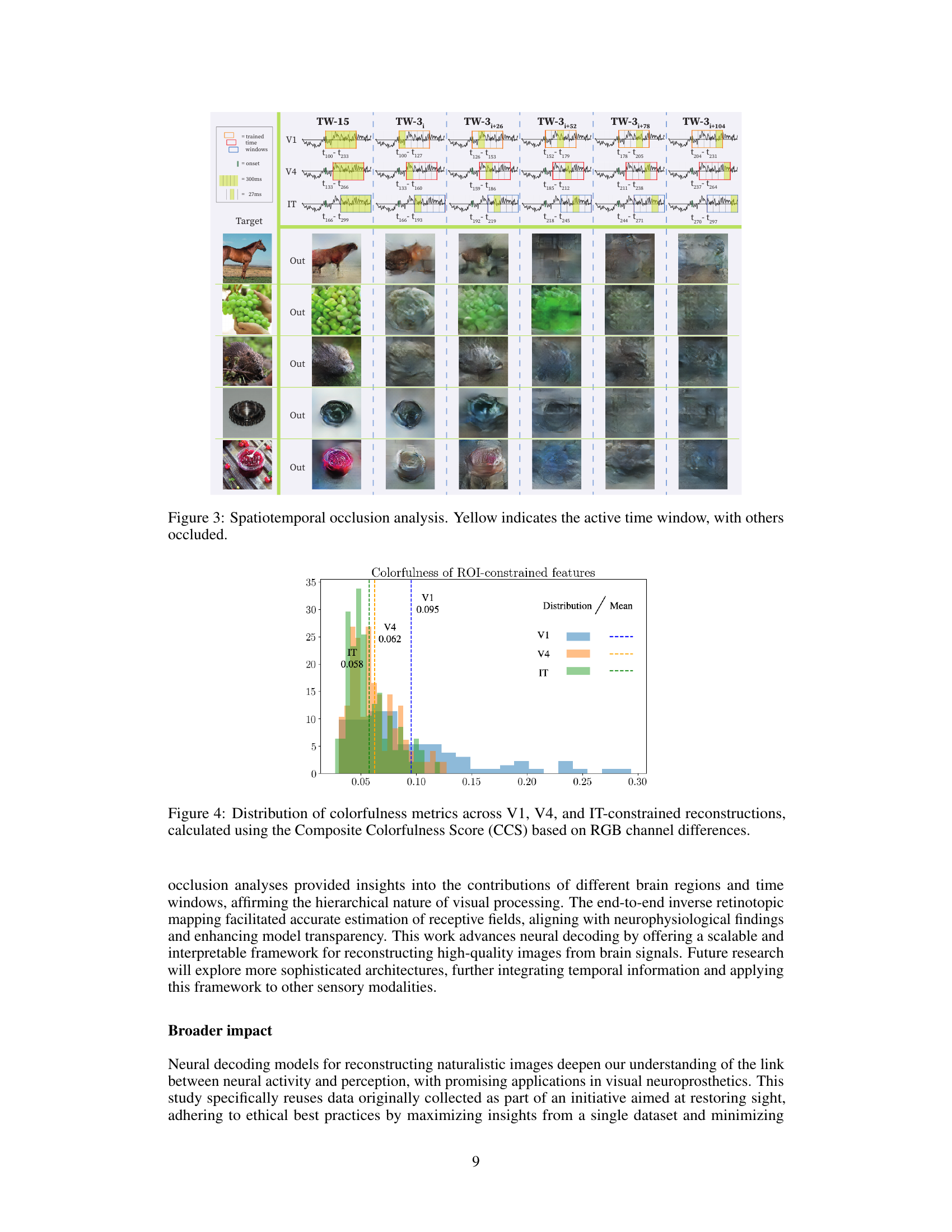
🔼 This figure demonstrates the results of a spatiotemporal occlusion analysis. Multiple example stimuli are shown, with their corresponding reconstructions when different time windows of neural responses are included or excluded in the model. Each column represents a different set of time windows being occluded, with the first column showing the reconstruction using all time windows. The yellow highlighted regions indicate which time windows’ data are used to reconstruct the image. This visualization is used to illustrate how different temporal components of neural activity contribute to the reconstruction of the visual stimuli.
read the caption
Figure 3: Spatiotemporal occlusion analysis. Yellow indicates the active time window, with others occluded.
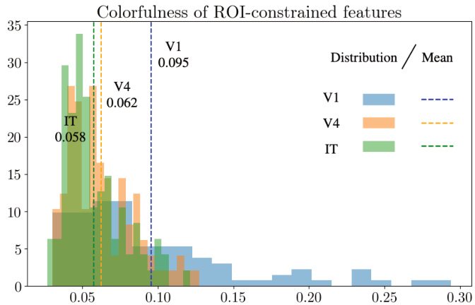
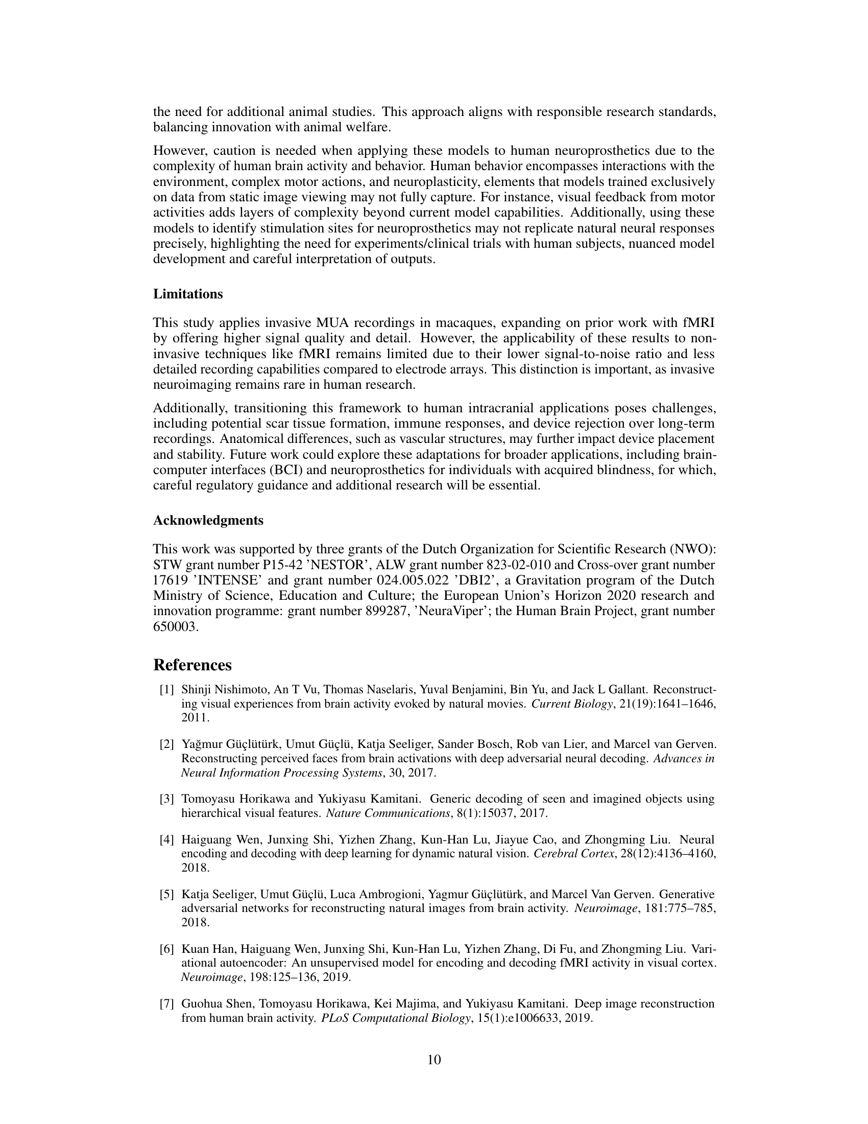
🔼 This histogram displays the distribution of colorfulness scores for image reconstructions derived from neural activity in three different brain regions (V1, V4, and IT). The colorfulness metric quantifies the perceptual quality of color in the images. The means for each region are displayed, showing a clear trend of increasing colorfulness from IT to V1, likely reflecting the hierarchical processing of color information in the visual cortex. The graph helps in visualizing the effect of restricting input to the reconstruction model to only a certain brain area.
read the caption
Figure 4: Distribution of colorfulness metrics across V1, V4, and IT-constrained reconstructions, calculated using the Composite Colorfulness Score (CCS) based on RGB channel differences.

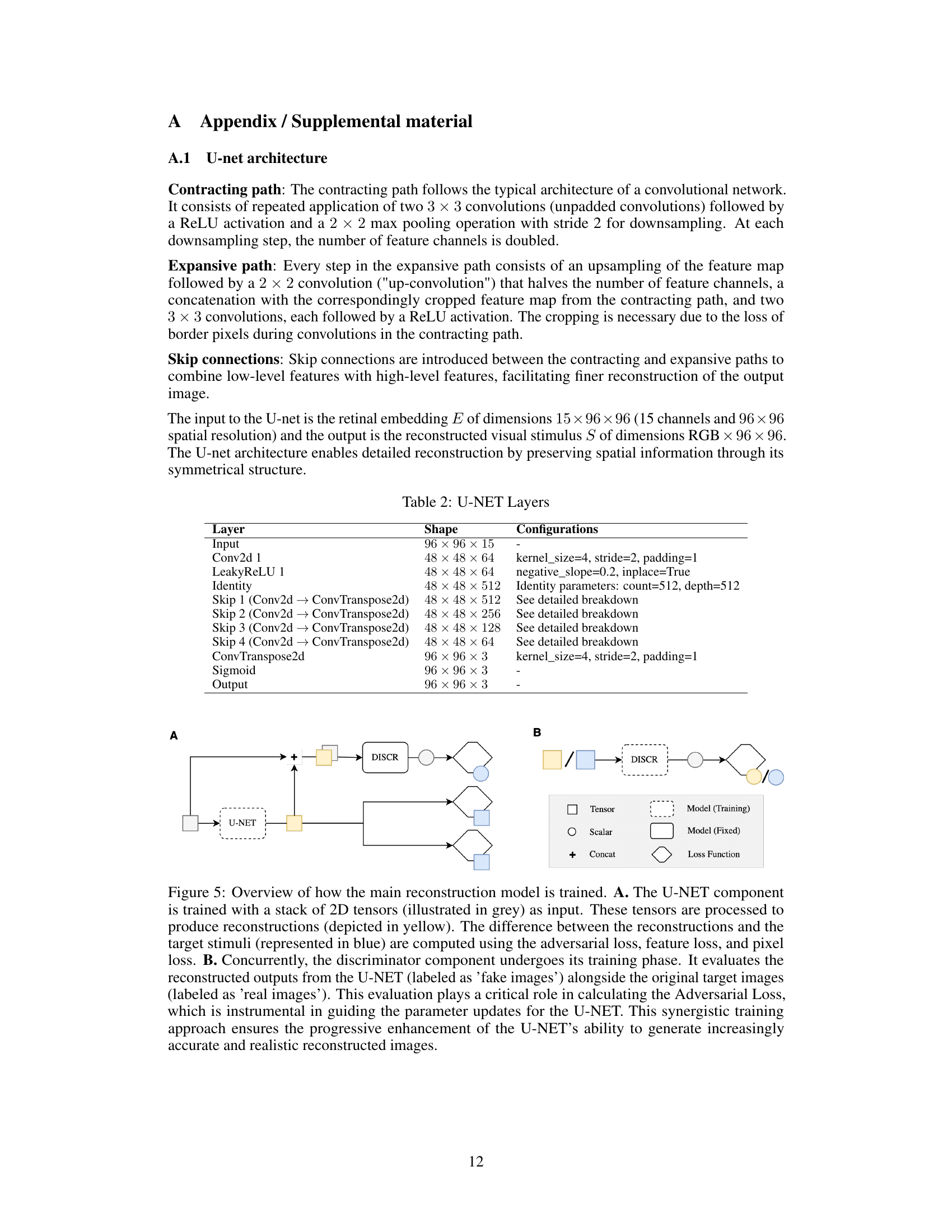
🔼 This figure shows the training process of the main reconstruction model which is a U-NET. The U-NET processes a stack of 2D tensors to produce reconstructions. The differences between the reconstructions and target stimuli are used to compute loss functions (adversarial, feature, and pixel loss). The discriminator evaluates reconstructed outputs and target images. This process helps the U-NET generate more accurate images.
read the caption
Figure 5: Overview of how the main reconstruction model is trained. A. The U-NET component is trained with a stack of 2D tensors (illustrated in grey) as input. These tensors are processed to produce reconstructions (depicted in yellow). The difference between the reconstructions and the target stimuli (represented in blue) are computed using the adversarial loss, feature loss, and pixel loss. B. Concurrently, the discriminator component undergoes its training phase. It evaluates the reconstructed outputs from the U-NET (labeled as 'fake images') alongside the original target images (labeled as 'real images'). This evaluation plays a critical role in calculating the Adversarial Loss, which is instrumental in guiding the parameter updates for the U-NET. This synergistic training approach ensures the progressive enhancement of the U-NET's ability to generate increasingly accurate and realistic reconstructed images.
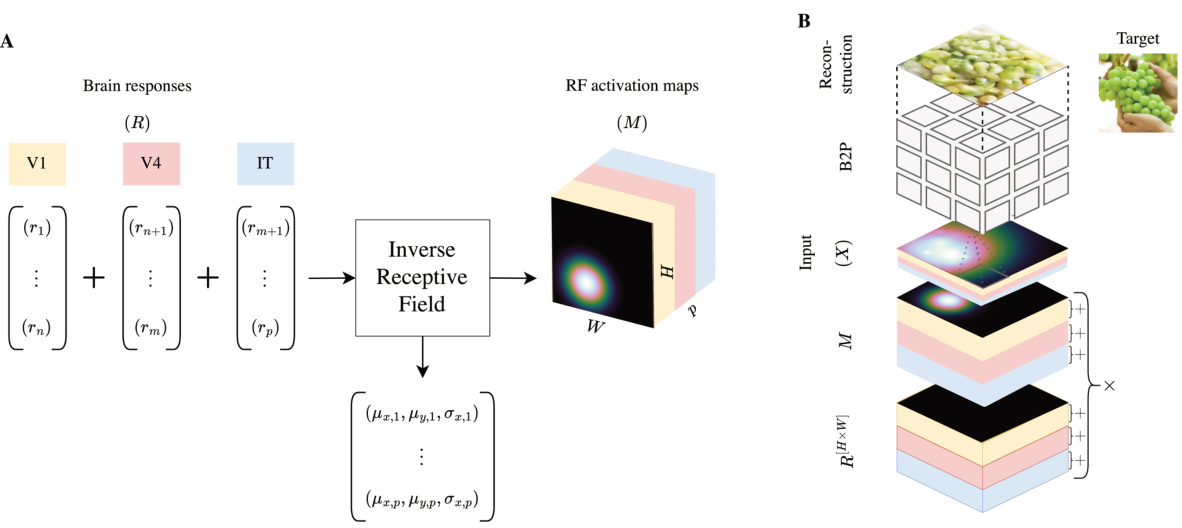
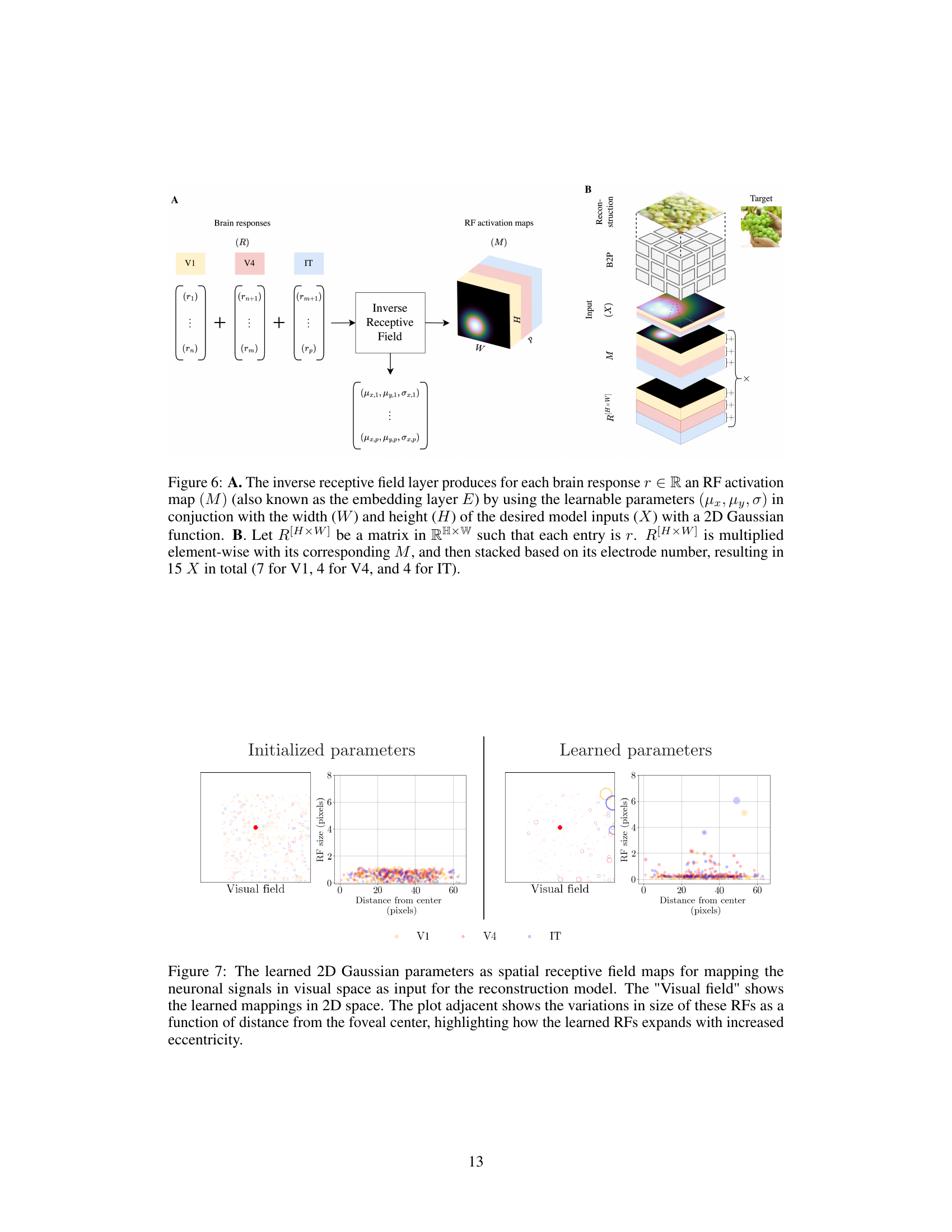
🔼 Figure 6 illustrates the process of the inverse receptive field layer in the homeomorphic decoder. Panel A shows the computation of the RF activation map (M) for each brain response r, using learnable parameters (µx, µy, σ) and a 2D Gaussian function. Panel B depicts how the brain responses (R), which are represented as a matrix R[H×W], are combined with their corresponding activation maps (M) and stacked based on electrode number to generate the final input for the decoder. The combination of responses from V1, V4 and IT areas results in a 15-channel input (7 from V1, 4 from V4, and 4 from IT).
read the caption
Figure 6: A. The inverse receptive field layer produces for each brain response r∈ R an RF activation map (M) (also known as the embedding layer E) by using the learnable parameters (μα, μy, σ) in conjunction with the width (W) and height (H) of the desired model inputs (X) with a 2D Gaussian function. B. Let R[H×W] be a matrix in RH×W such that each entry is r. R[H×W] is multiplied element-wise with its corresponding M, and then stacked based on its electrode number, resulting in 15 X in total (7 for V1, 4 for V4, and 4 for IT).

🔼 This figure shows the learned receptive fields (RFs) of the model, visualizing how the model learned to map neuronal signals to spatial locations in the visual field. The left panel shows the spatial distribution of the receptive fields, while the right panel shows how the size of the receptive fields changes with distance from the center of the visual field (fovea). Different colors represent different brain regions (V1, V4, IT).
read the caption
Figure 7: The learned 2D Gaussian parameters as spatial receptive field maps for mapping the neuronal signals in visual space as input for the reconstruction model. The 'Visual field' shows the learned mappings in 2D space. The plot adjacent shows the variations in size of these RFs as a function of distance from the foveal center, highlighting how the learned RFs expands with increased eccentricity.
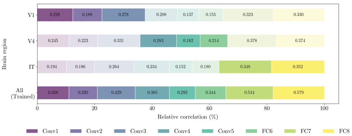
🔼 This figure displays the relative correlation coefficients between features extracted from reconstructed images (using only V1, V4, IT, and all brain regions) and features from different layers of a pre-trained AlexNet model. The relative correlations are normalized for each brain region, allowing direct comparison across regions and layers. Higher correlations are indicated by deeper colors and larger bar heights, visually highlighting which ROI reconstruction best aligns with specific processing stages within AlexNet.
read the caption
Figure 8: Relative correlation analysis of ROI-constrained reconstructions with AlexNet features. This figure shows the relative correlation coefficients between features from ROI-constrained reconstructions (V1, V4, IT) and corresponding AlexNet layers, normalized per brain region for fair comparison. Higher relative correlations are indicated by deeper colors and larger bars, marking the ROI reconstruction with the closest match to each AlexNet layer's processing characteristics.
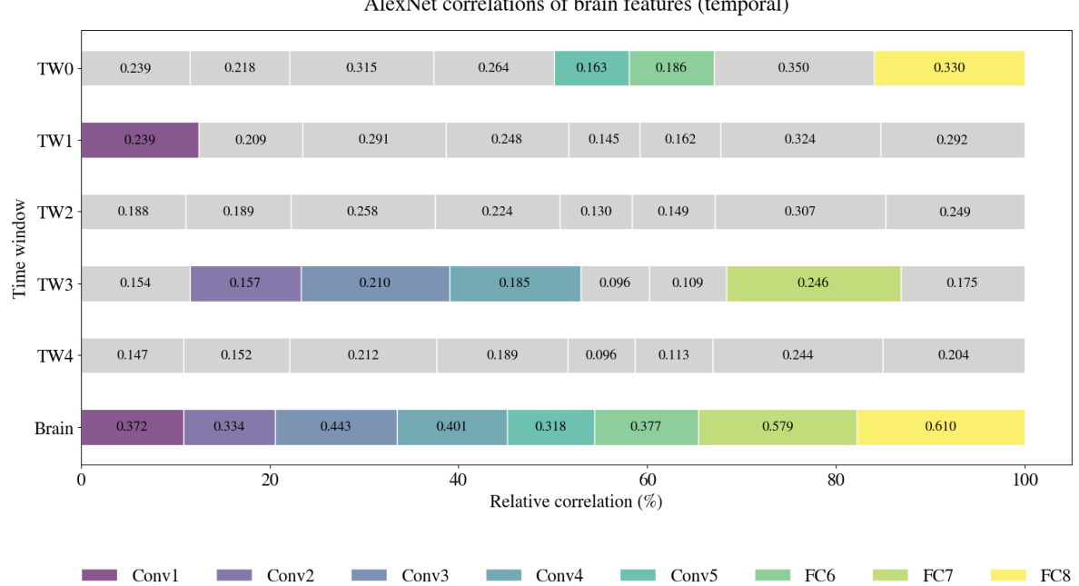
🔼 This figure shows the relative correlation coefficients between features from reconstructions at different time windows and various AlexNet layers. The color intensity and bar length represent the strength of the correlation, normalized per brain region for easier comparison. The x-axis is normalized, enabling a direct comparison of the relative contributions across different time points.
read the caption
Figure 9: Temporal relative correlation analysis across AlexNet layers. This figure illustrates relative correlation coefficients across multiple time windows and AlexNet layers, with color and bar size representing the highest relative (not absolute) correlations per brain region. The x-axis is normalized, allowing direct comparison of relative contributions across time points.
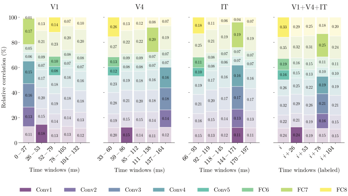
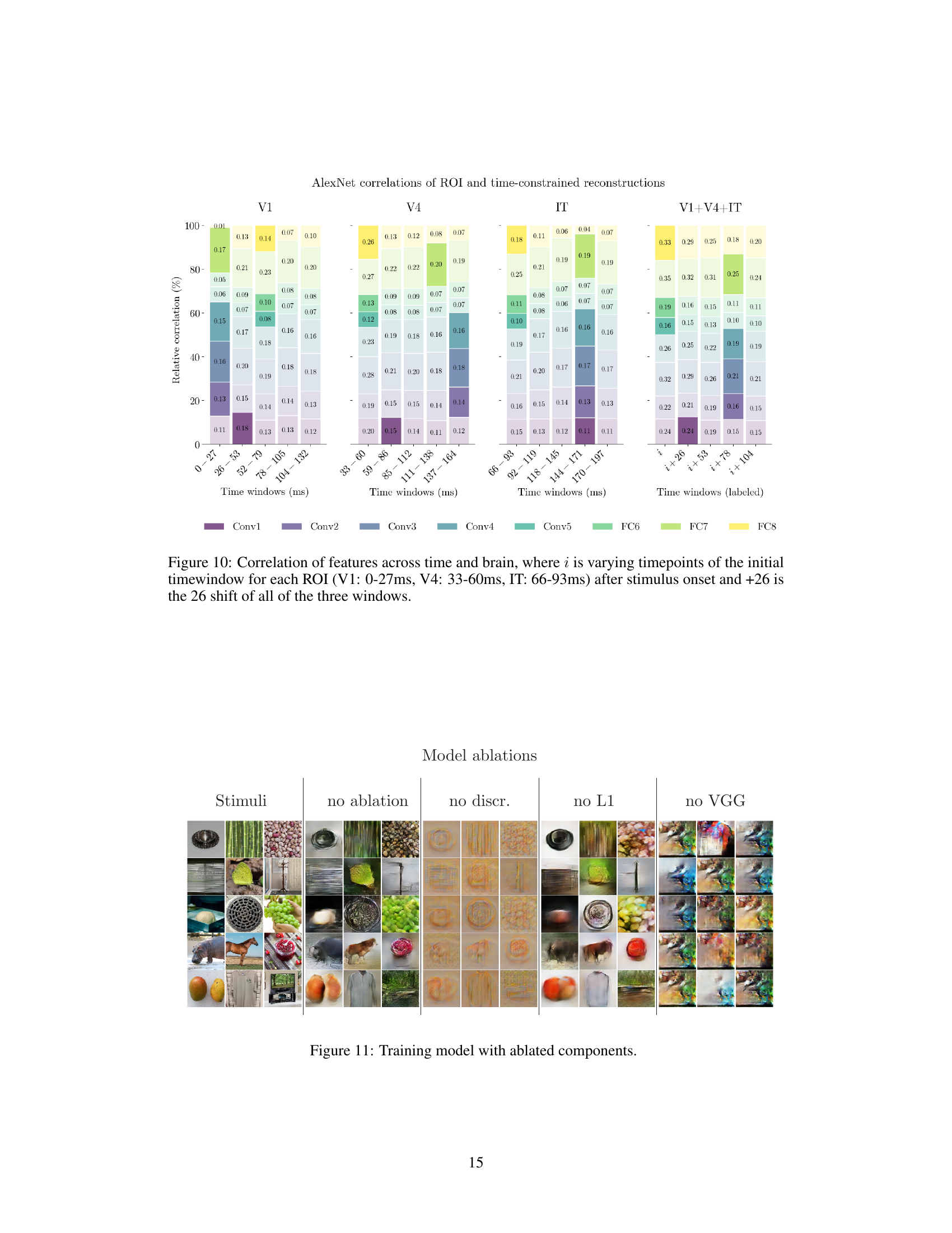
🔼 This figure shows the correlation of features across different time windows and brain regions (V1, V4, IT). It demonstrates how the relative contribution of each brain region changes over time in reconstructing visual stimuli. The varying time windows after stimulus onset are represented (0-27ms for V1, 33-60ms for V4, 66-93ms for IT) and subsequent 26ms shifts. The higher correlations are indicated by deeper colors and larger bars.
read the caption
Figure 10: Correlation of features across time and brain, where i is varying timepoints of the initial timewindow for each ROI (V1: 0-27ms, V4: 33-60ms, IT: 66-93ms) after stimulus onset and +26 is the 26 shift of all of the three windows.
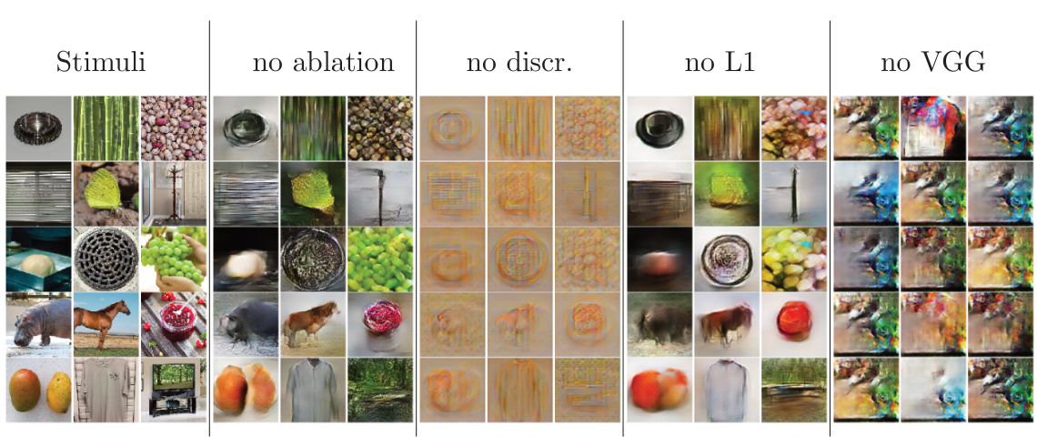
🔼 This figure shows the impact of removing different components from the training model on the quality of the reconstructed images. The columns represent different model variations: no ablation (full model), no discriminator, no L1 loss, and no VGG loss. Each row represents a different stimulus image, with the corresponding reconstructions shown in each column. Comparing the reconstructions across different columns helps visualize the role of each component in the model’s performance.
read the caption
Figure 11: Training model with ablated components.

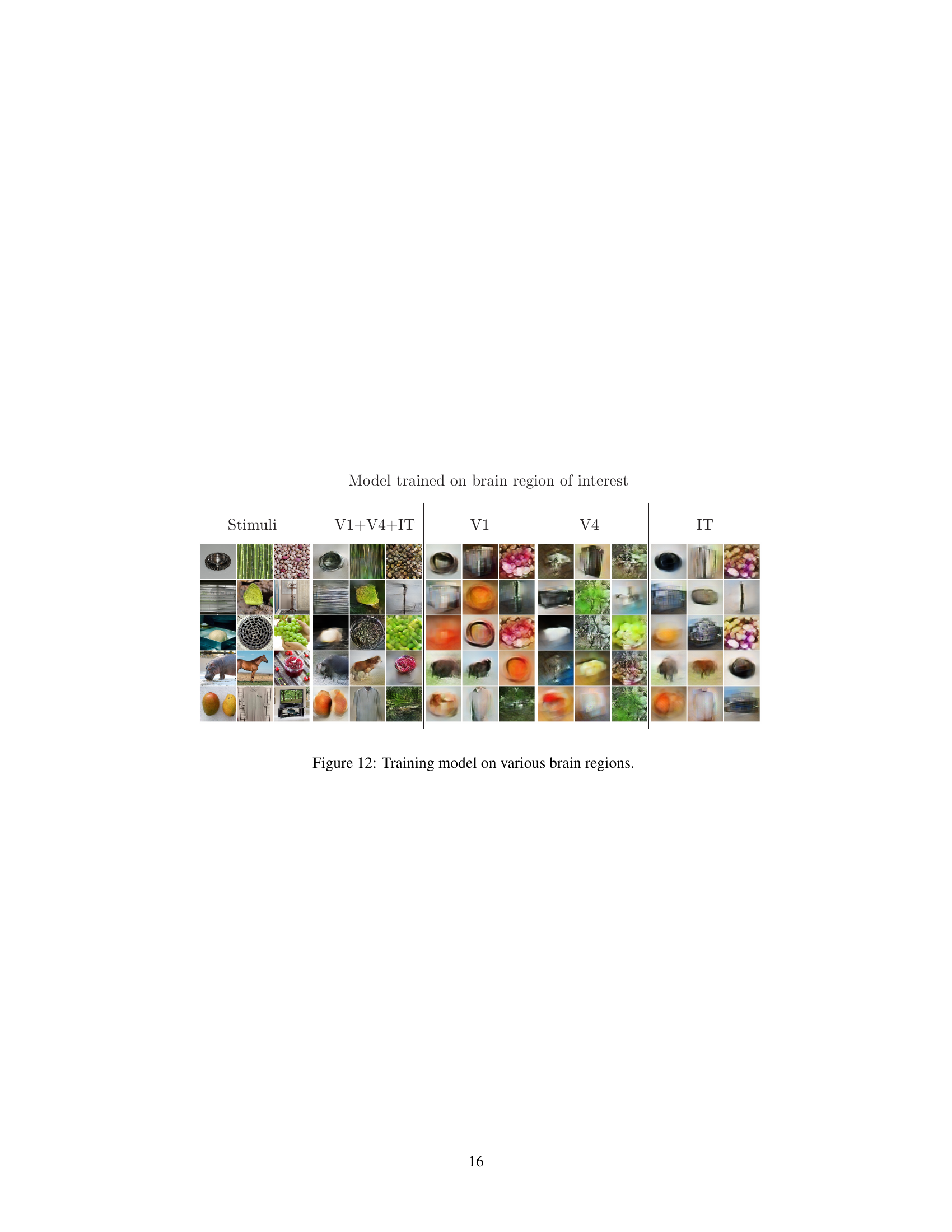
🔼 This figure shows the results of training the model on different brain regions (V1, V4, IT, and V1+V4+IT). Each column represents a different brain region used for training, and each row displays reconstructed images corresponding to a specific input stimulus from the THINGS dataset. By comparing the reconstructed images across different brain regions, the figure aims to demonstrate the impact of the source brain region on the quality and features of the reconstructed images, highlighting the region-specific contributions to image reconstruction.
read the caption
Figure 12: Training model on various brain regions.
Full paper#

