TL;DR#
Generative models excel at creating static 3D geometric structures, but struggle with dynamic systems. Modeling dynamic systems is challenging due to the complex interplay of spatial interactions and temporal correspondence, along with the need to maintain physical symmetries. Existing methods fail to capture this temporal aspect, limiting their applicability.
GeoTDM successfully addresses this limitation by introducing a novel diffusion model that generates high-quality geometric trajectories. This involves a new transition kernel that leverages SE(3)-equivariant spatial convolution and temporal attention. The model is also enhanced with a generalized learnable geometric prior for improved temporal conditioning. GeoTDM significantly outperforms existing methods in various generation scenarios, demonstrating its effectiveness and setting a new standard for generating dynamic geometric data.
Key Takeaways#
Why does it matter?#
This paper is crucial because it introduces GeoTDM, the first diffusion model for generating realistic 3D geometric trajectories. This addresses a significant gap in existing generative models, which primarily focus on static structures. Its impact extends to various fields, including molecular dynamics, robotics, and computer graphics, opening new avenues for research and applications in modeling dynamic systems.
Visual Insights#

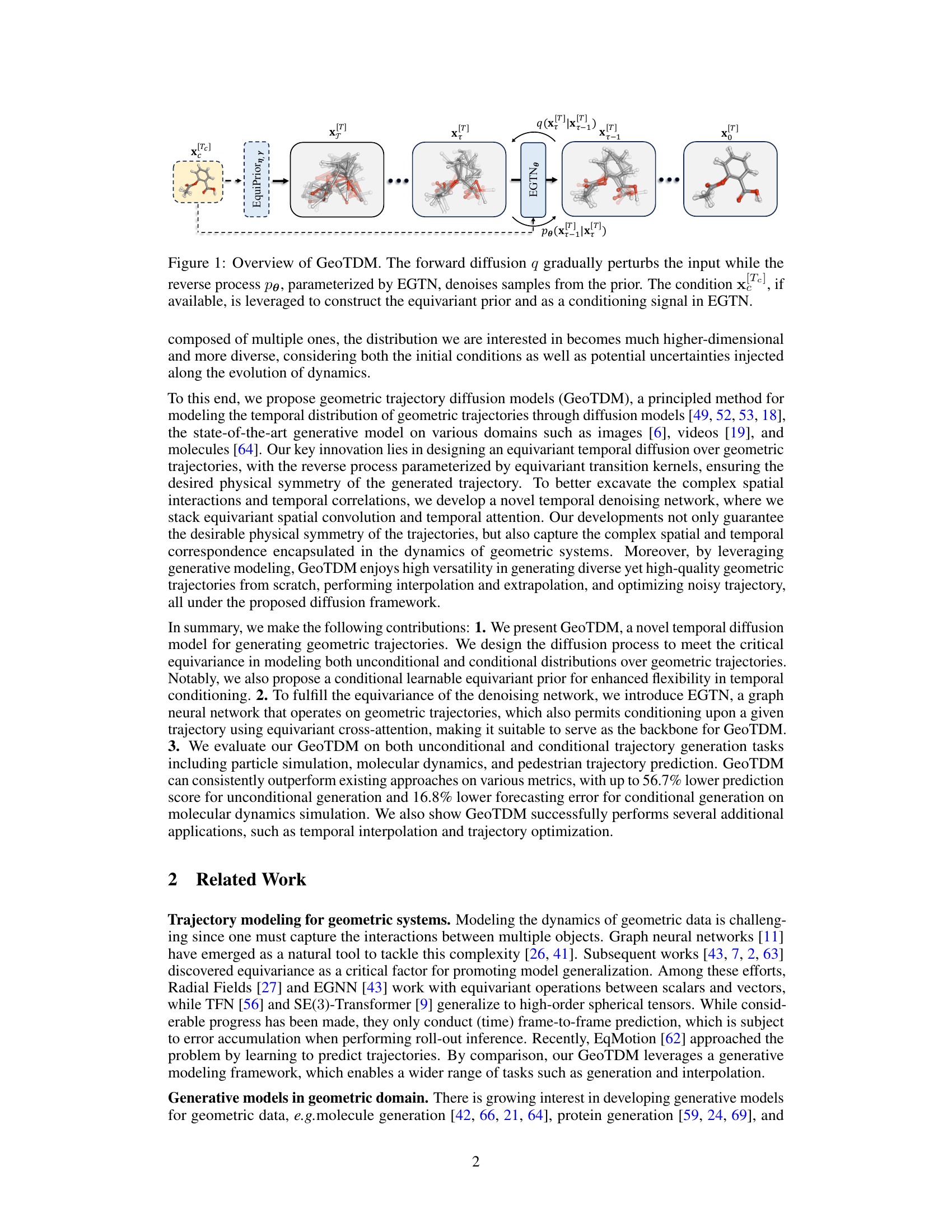
🔼 This figure provides a high-level overview of the GeoTDM model. It shows how the forward diffusion process adds noise to the input data step-by-step, and the reverse process uses the EGTN (Equivariant Geometric Trajectory Network) to remove the noise and generate samples from a learned prior distribution. The process is shown for both unconditional and conditional generation, indicating how conditional information can influence the generation process via the equivariant prior and as a signal within EGTN.
read the caption
Figure 1: Overview of GeoTDM. The forward diffusion q gradually perturbs the input while the reverse process pθ, parameterized by EGTN, denoises samples from the prior. The condition x, if available, is leveraged to construct the equivariant prior and as a conditioning signal in EGTN.

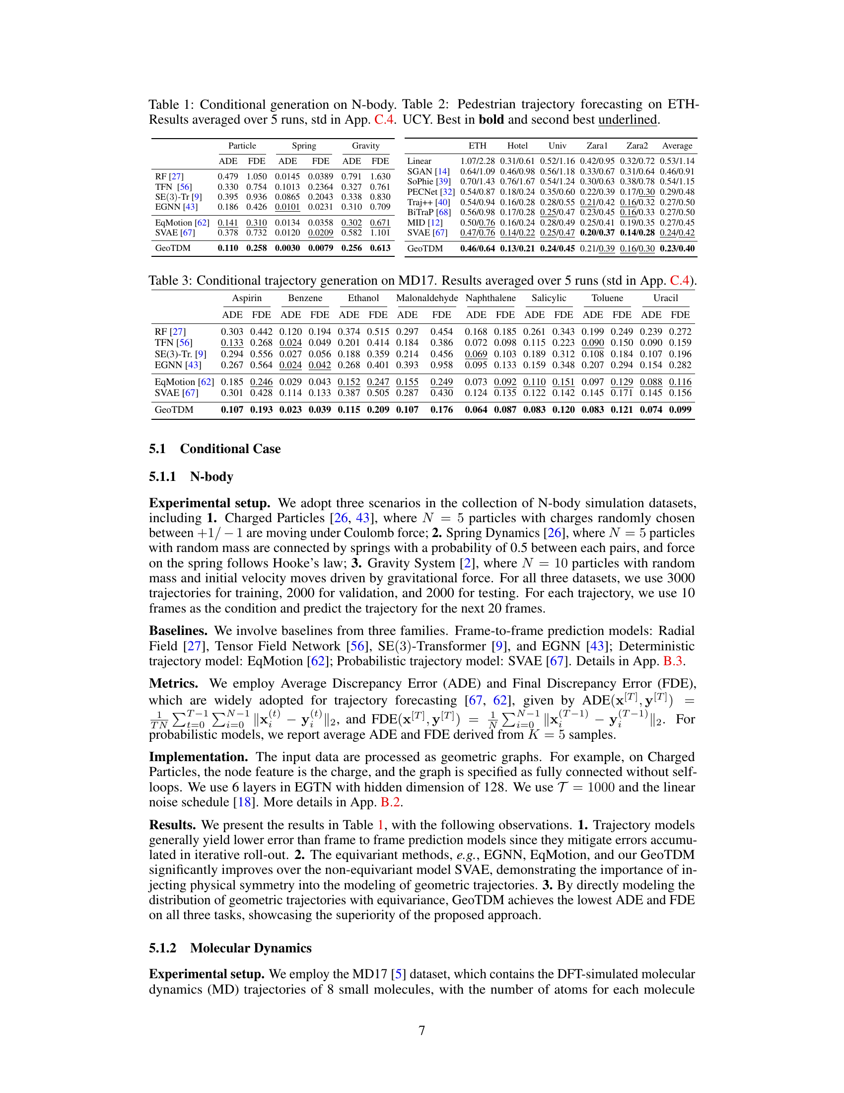
🔼 This table presents the results of conditional trajectory generation experiments on three different N-body simulation datasets: Charged Particles, Spring Dynamics, and Gravity System. The table compares GeoTDM’s performance against several baselines across different metrics (ADE and FDE). The results are averaged over 5 runs, and standard deviations are provided in Appendix C.4. The best-performing method for each dataset and metric is shown in bold, with the second-best underlined.
read the caption
Table 1: Conditional generation on N-body. Results averaged over 5 runs, std in App. C.4. UCY. Best in bold and second best underlined.
In-depth insights#
Equivariant Diffusion#
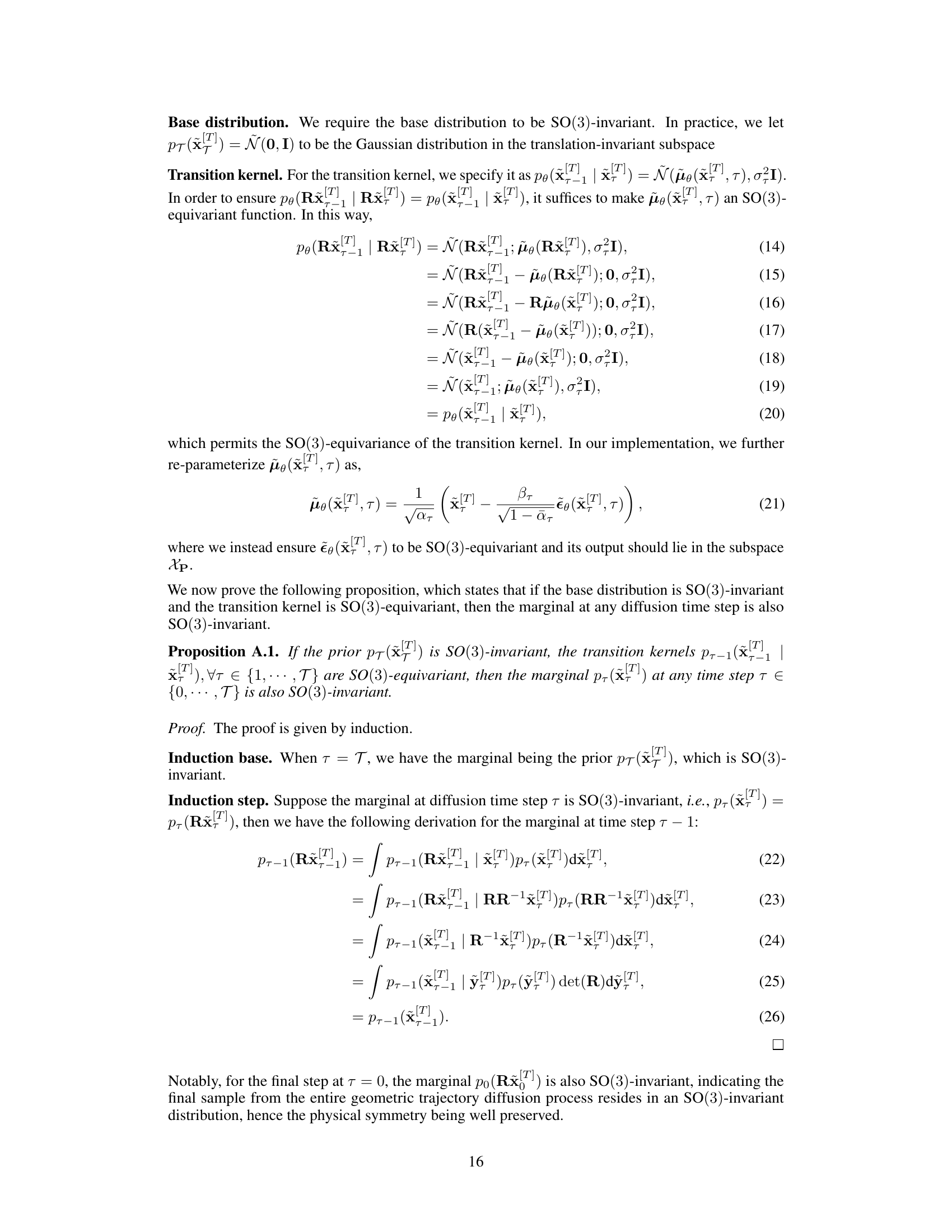
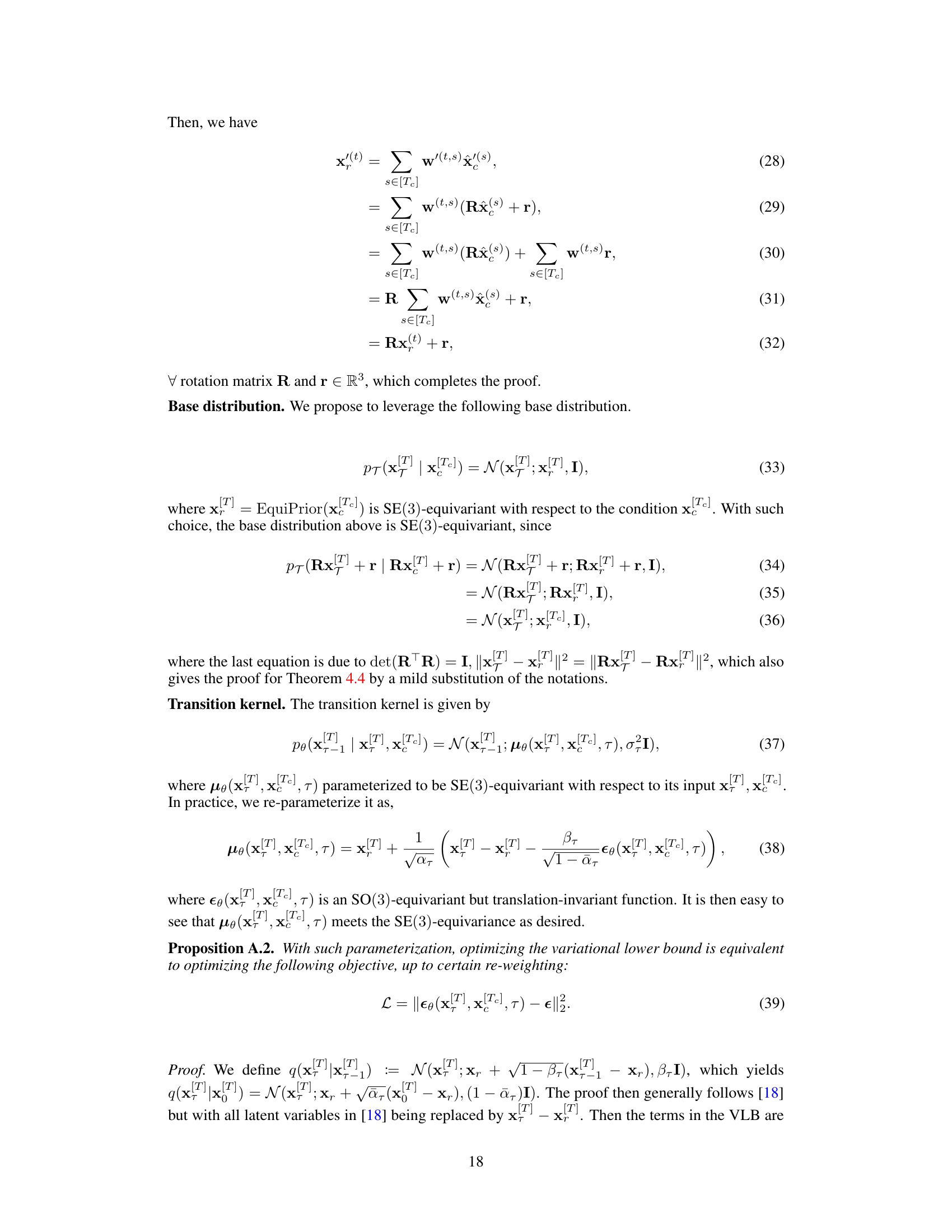
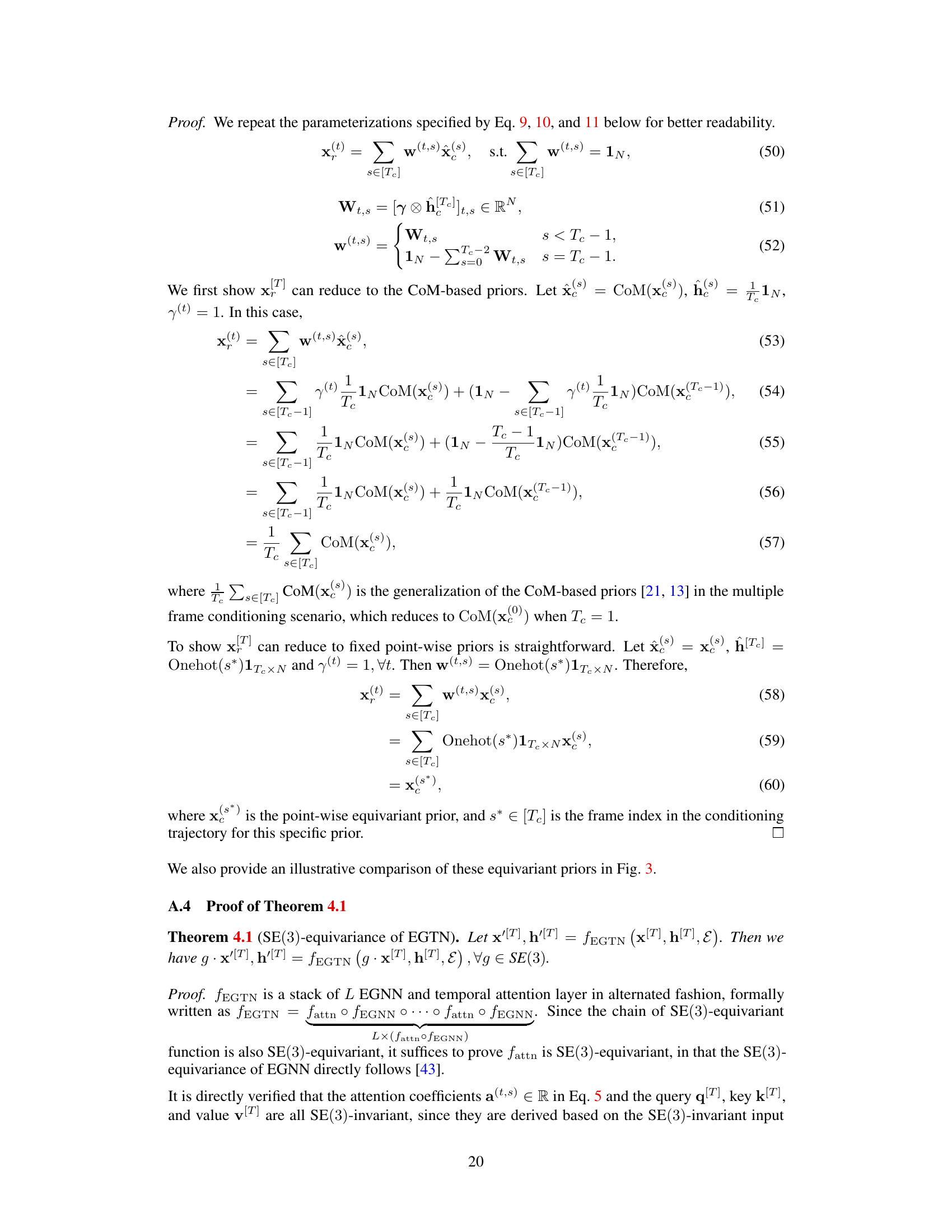
Equivariant diffusion models represent a significant advancement in generative modeling, particularly for data exhibiting inherent symmetries, such as those found in molecular structures or physical systems. Equivariance ensures that if the input data is transformed (e.g., rotated or translated), the output of the model undergoes a corresponding transformation, maintaining consistency in the generated data. This is crucial for generating realistic and physically meaningful outputs, unlike traditional diffusion models which might produce nonsensical results when such transformations are applied. The key advantage lies in the model’s ability to capture and leverage symmetries directly within its architecture, leading to more efficient learning and improved generalization. This often involves utilizing specialized layers or network designs that explicitly incorporate these symmetries, often employing group theory principles. While standard diffusion models excel at generating diverse data, equivariant variants guarantee this diversity within the constraints of the underlying symmetries; essential for tasks like molecule design or fluid simulation where preserving physical properties is vital. The increased computational cost is often offset by the superior quality and coherence of the generated data, making it a valuable tool for diverse scientific and engineering applications.
Geometric Trajectory#
The concept of ‘Geometric Trajectory’ in a research paper likely refers to the mathematical representation and analysis of the movement of geometric objects over time. This could involve studying trajectories of points, curves, or even more complex shapes in various dimensional spaces. The focus might be on describing the trajectory’s shape, its evolution, or its properties like smoothness or curvature. Key aspects likely explored are the trajectory’s underlying dynamics (physical laws, forces, or constraints governing motion), and potentially the development of algorithms for trajectory prediction or generation, perhaps employing machine learning techniques. Such a study would likely involve sophisticated mathematical frameworks, likely including differential geometry, topology, or group theory. Applications of this research could span diverse fields, such as robotics (planning robot movements), computer graphics (animating objects realistically), or even physics (simulating the movement of particles). The study might also delve into the relationship between geometric properties of the trajectory and other factors, perhaps discovering correlations or causations. Furthermore, any work in this area would need to consider computational challenges associated with handling complex geometric data and potentially high-dimensional spaces.
Temporal Denoising#
Temporal denoising in the context of a research paper likely involves techniques designed to remove noise or artifacts from temporal data, such as time series or video sequences. This would be crucial for applications where preserving temporal fidelity is important. Effective temporal denoising likely needs to consider the correlation structure of the data over time. Simple methods that operate on individual frames independently might fail to capture this. Advanced techniques might use recurrent neural networks (RNNs), convolutional neural networks (CNNs) operating over time, or diffusion models to learn and model the temporal dependencies. A key challenge is to differentiate between true signal and noise, especially when dealing with complex or dynamic systems. Successful methods will also be computationally efficient, allowing application to large datasets. The effectiveness will likely be evaluated with metrics measuring temporal accuracy (e.g., mean squared error) and preserving the underlying dynamics.
Conditional Generation#
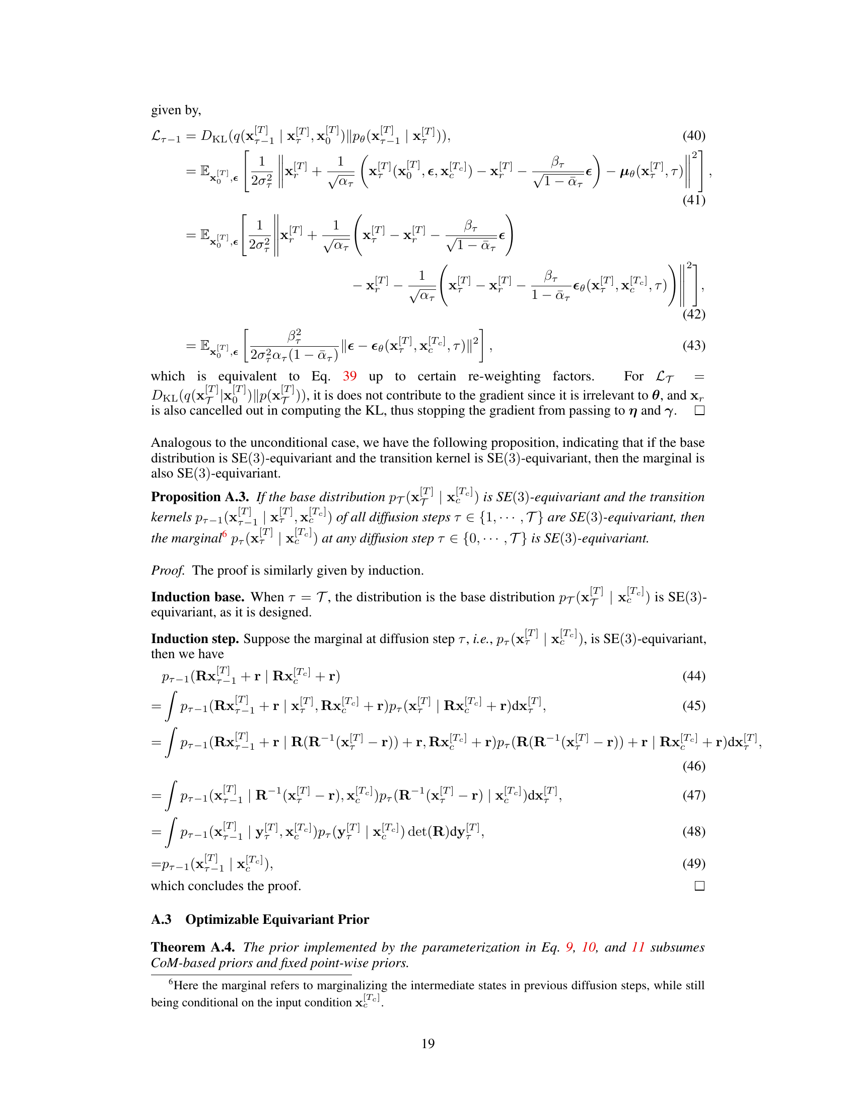
Conditional generation, in the context of geometric trajectory diffusion models, focuses on generating trajectories given some prior knowledge or constraints. Instead of creating trajectories from scratch, this approach leverages existing trajectory data as a conditioning signal to guide the generation process. This is particularly important for applications where some portion of the trajectory is already known or observed. The key challenge lies in designing a system that maintains the physical symmetries and temporal correlations inherent in geometric systems while incorporating this conditional information. This requires carefully designed methods that leverage the conditioning data while ensuring the model generates realistic and physically plausible trajectories. For example, in molecular dynamics, the conditioning might be an initial molecular configuration, influencing the generation of subsequent movements. Successful conditional generation in this domain would enable simulating complex molecular dynamics based on partial data, significantly enhancing the modeling capabilities of such systems. The successful implementation of conditional generation hinges on equivariant mechanisms that ensure the model appropriately transforms the conditioning and generated data, maintaining the consistency of the physical laws underlying the geometric process.
Ablation Studies#
Ablation studies systematically remove components of a model to assess their individual contributions. In the context of a research paper, a well-designed ablation study would isolate and test the impact of key elements, such as specific layers in a neural network, specific components of a loss function, or other architectural design choices. The goal is to demonstrate the necessity and effectiveness of each component, showing that removing it leads to a measurable decline in performance. This process helps establish the causal relationship between the model’s design and its performance. Well-executed ablation studies can help build trust and understanding by showing precisely what is driving the model’s success. They can also lead to design improvements by revealing which components are most critical or redundant. However, the interpretation of ablation studies requires careful consideration. It is important to ensure that the removed components don’t interact unexpectedly with others, invalidating the conclusions. Furthermore, the ablation approach should align with the model’s overall design philosophy. A comprehensive ablation study would explore a variety of design choices and their impact, ideally with various experimental settings or datasets, enabling researchers to extract more robust and reliable findings.
More visual insights#
More on figures

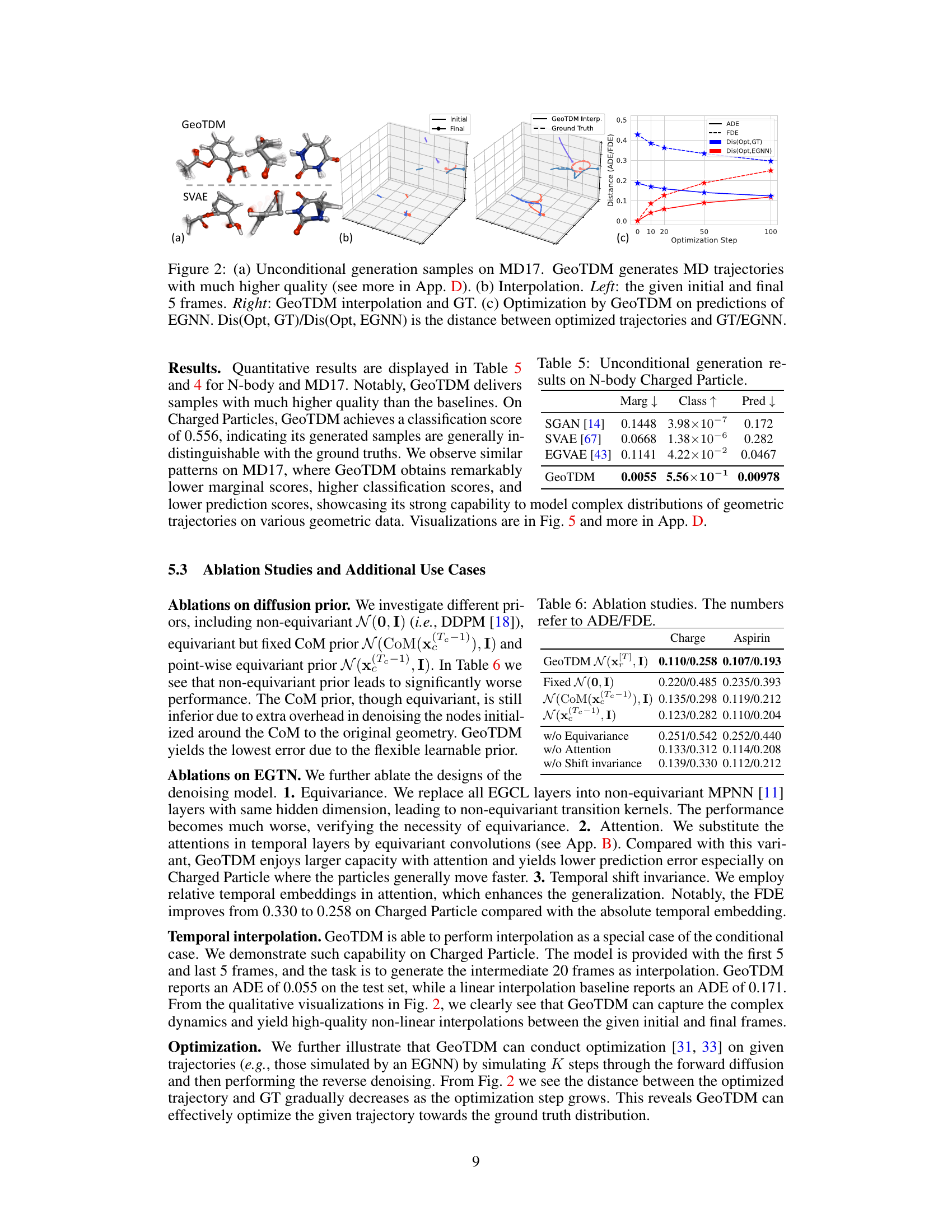
🔼 This figure demonstrates the performance of GeoTDM in three different scenarios: unconditional generation, interpolation, and optimization. (a) Shows that GeoTDM generates higher-quality molecular dynamics (MD) trajectories compared to other baselines. (b) Illustrates GeoTDM’s ability to interpolate between given initial and final frames, capturing the dynamics in between. (c) Shows that GeoTDM can effectively optimize trajectories generated by another model (EGNN), moving them closer to the ground truth.
read the caption
Figure 2: (a) Unconditional generation samples on MD17. GeoTDM generates MD trajectories with much higher quality (see more in App. D). (b) Interpolation. Left: the given initial and final 5 frames. Right: GeoTDM interpolation and GT. (c) Optimization by GeoTDM on predictions of EGNN. Dis(Opt, GT)/Dis(Opt, EGNN) is the distance between optimized trajectories and GT/EGNN.

🔼 This figure illustrates three different types of equivariant priors used in the Geometric Trajectory Diffusion Models (GeoTDM) for conditional generation. The CoM-based prior uses the center of mass of the conditioning trajectory as the mean of the prior distribution. The fixed point-wise prior uses a single frame from the conditioning trajectory as the prior. The GeoTDM’s prior uses a learned weighted combination of the conditioning trajectory to form a flexible prior that incorporates both spatial and temporal information.
read the caption
Figure 3: An illustration of different equivariant priors. For simplicity in the chart here we only illustrate the case when N = 3 and T_c = 1, T = 1.
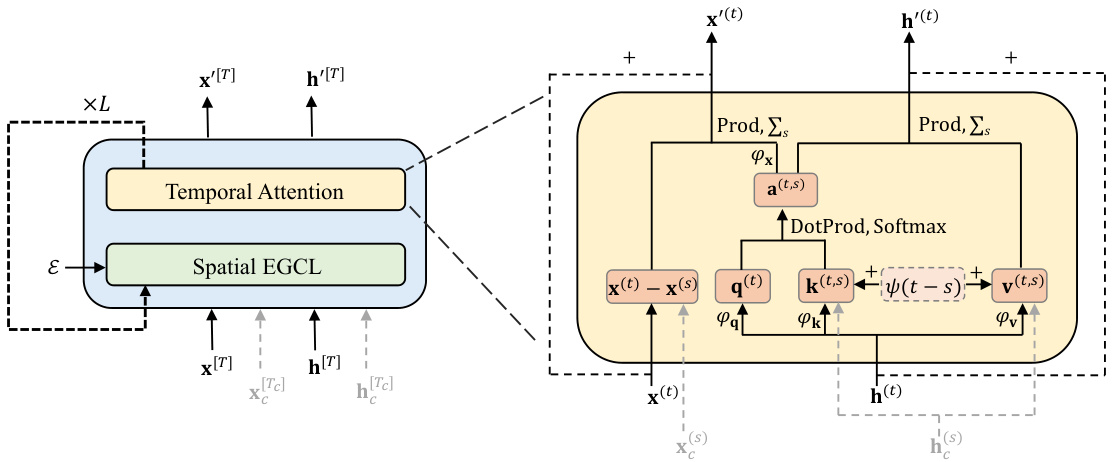
🔼 This figure shows the architecture of the Equivariant Geometric Trajectory Network (EGTN). The network alternates between equivariant spatial aggregation layers (EGCL) and temporal attention layers. EGCL layers process spatial interactions within each timestep, while temporal attention layers model temporal dependencies across timesteps. The network also incorporates a mechanism for incorporating conditional information (x[Tc], hc) via cross-attention, using a relative positional encoding (t-s) for better capturing temporal correlation. The overall process is designed to ensure SE(3) equivariance, preserving the physical symmetry properties during generation.
read the caption
Figure 4: Schematic of the proposed EGTN, which alternates the EGCL layer for extracting spatial interactions and the temporal attention layer for modeling temporal sequence. Additional conditional information x[Tc] and hc can also be processed using cross-attention. The relative temporal embedding (t – s) is added to the key and value. DotProd refers to dot product and Softmax is performed over indexes of s.
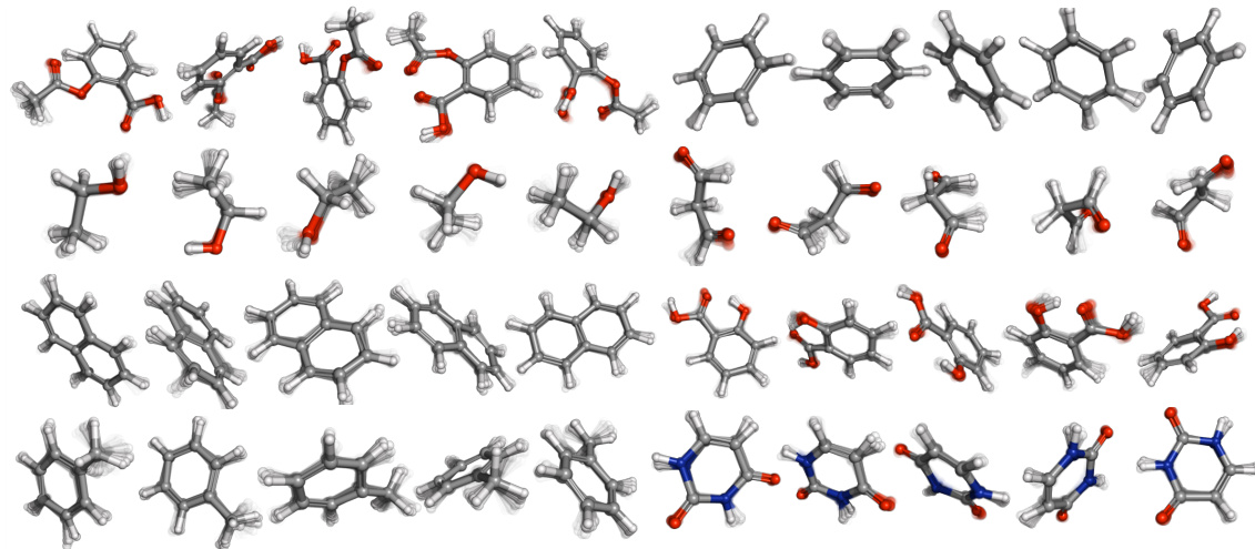
🔼 This figure shows uncurated samples generated by GeoTDM on the MD17 dataset for unconditional generation. It displays trajectories for eight different molecules, highlighting GeoTDM’s ability to generate high-quality samples that accurately capture molecular vibrations and rotations.
read the caption
Figure 5: Uncurated samples of GeoTDM on MD17 dataset in the unconditional generation setup. From top-left to bottom-right are trajectories of the eight molecules: Aspirin, Benzene, Ethanol, Malonaldehyde, Naphthalene, Salicylic, Toluene, and Uracil. Five samples are displayed for each molecule. GeoTDM generates high quality samples. It well captures the vibrations and rotating behavior of the methyl groups in Aspirin and Ethanol. The bonds on the benzene ring are also more stable, aligning with findings in chemistry.

🔼 This figure shows uncurated samples generated by GeoTDM for eight different molecules in the MD17 dataset. The model successfully captures the complex vibrational and rotational movements of these molecules, particularly highlighting the accurate representation of methyl groups and benzene rings.
read the caption
Figure 5: Uncurated samples of GeoTDM on MD17 dataset in the unconditional generation setup. From top-left to bottom-right are trajectories of the eight molecules: Aspirin, Benzene, Ethanol, Malonaldehyde, Naphthalene, Salicylic, Toluene, and Uracil. Five samples are displayed for each molecule. GeoTDM generates high quality samples. It well captures the vibrations and rotating behavior of the methyl groups in Aspirin and Ethanol. The bonds on the benzene ring are also more stable, aligning with findings in chemistry.
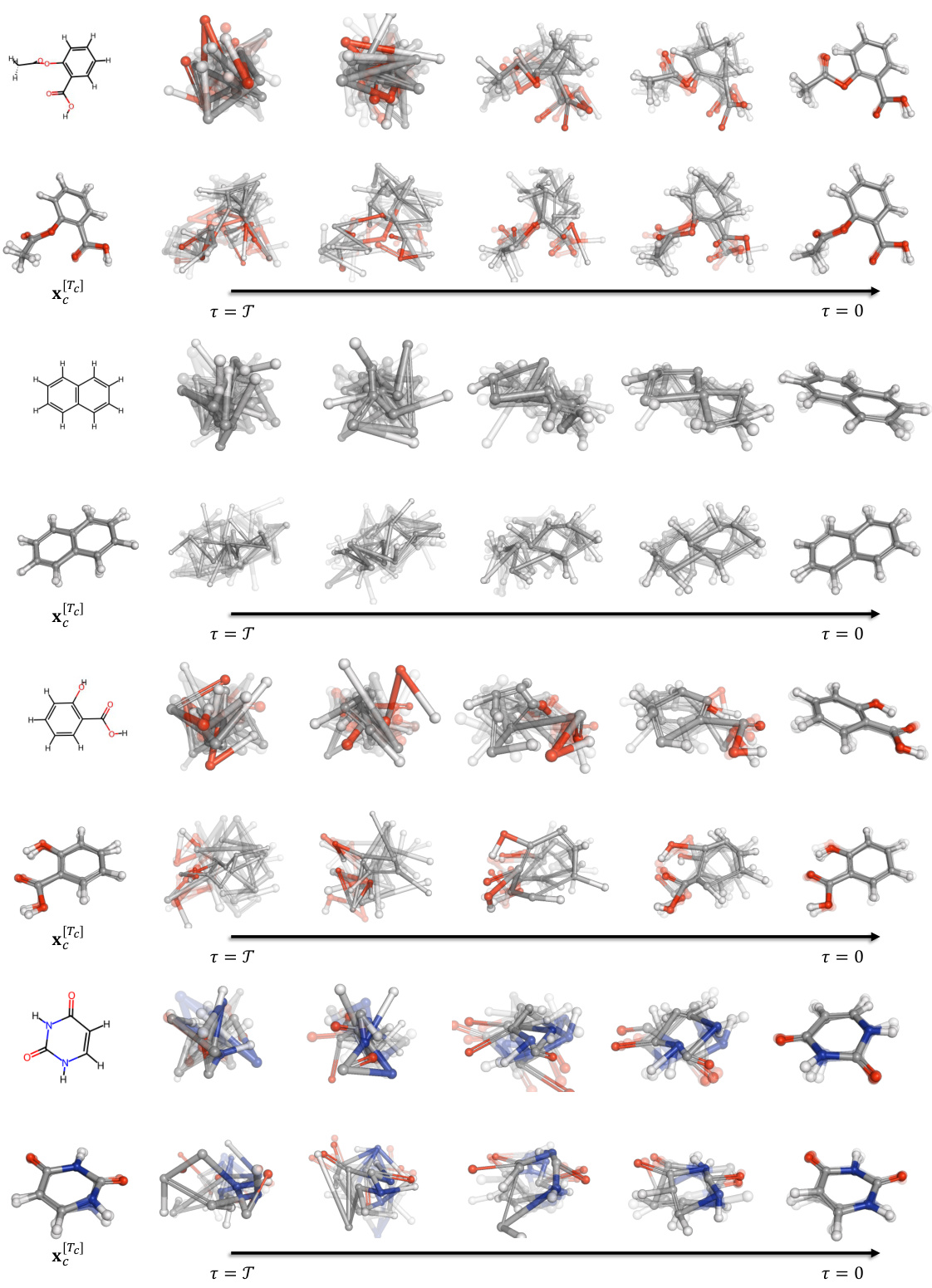
🔼 This figure visualizes the diffusion process of four different molecules (Aspirin, Naphthalene, Salicylic, and Uracil) at different diffusion steps (τ). The top row shows unconditional generation, starting from an invariant prior based solely on the molecule’s graph structure. The bottom row shows conditional generation, incorporating the equivariant prior conditioned on some given frames of the trajectory. It highlights how the equivariant prior retains structural information even after the diffusion process.
read the caption
Figure 7: Visualization of the diffusion trajectory at different diffusion steps. From top to bottom: Aspirin, Naphthalene, Salicylic, Uracil. For each molecule, the first row shows the unconditional generation process, where the model generates the trajectory from the invariant prior purely from the molecule graph without any conditioning structure. The second row refers to the conditional generation, where the model generates from the equivariant prior, conditioning on some given frames x[Tc]. Notably, the equivariant prior (see samples at τ = T in each second row) preserves some structural information encapsulated in x[Tc], thanks to our flexible parameterization.
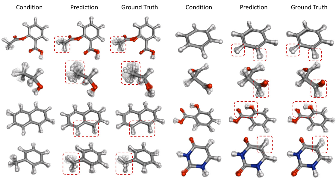
🔼 This figure shows some uncurated samples of the GeoTDM model on the MD17 dataset for the conditional forecasting setting. The model successfully generates samples with high accuracy, while also capturing some of the stochasticity inherent in molecular dynamics. Specific regions of interest are highlighted to emphasize the detail and accuracy of the generated samples.
read the caption
Figure 8: Uncurated samples of GeoTDM on MD17 dataset in the conditional forecasting setting. We highlight some regions of interest in red dashed boxes. GeoTDM delivers samples with very high accuracy while also capturing some stochasticity of the molecular dynamics.

🔼 This figure compares the generated samples of GeoTDM and a VAE model on the Charged Particles dataset. It visually demonstrates the quality difference between the two models in generating trajectories of charged particles in three dimensions. The color of the nodes indicates the charge of the particles (+1 in red, -1 in blue). The figure highlights GeoTDM’s ability to better capture the complex, realistic dynamics of the particles compared to the VAE. The data samples, GeoTDM predictions, and VAE predictions are presented for visual comparison.
read the caption
Figure 9: Visualization of data samples and generated samples by GeoTDM and SVAE in the unconditional setting on Charged Particles dataset. Nodes with color red and blue have the charge of +1/-1, respectively. Best viewed by zooming in.
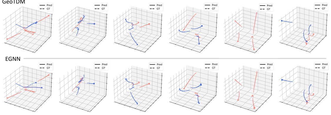
🔼 This figure compares the prediction results of GeoTDM and EGNN on the Charged Particles dataset in a conditional setting. Each subfigure shows a single prediction made by each model, along with the corresponding ground truth trajectory. The figure highlights the differences in predictive accuracy between the two methods and how well they capture the dynamics of the charged particles.
read the caption
Figure 10: Visualization of predictions by GeoTDM and EGNN in the conditional setting on Charged Particles dataset. Nodes with color red and blue have the charge of +1/-1, respectively. Best viewed by zooming in.
More on tables

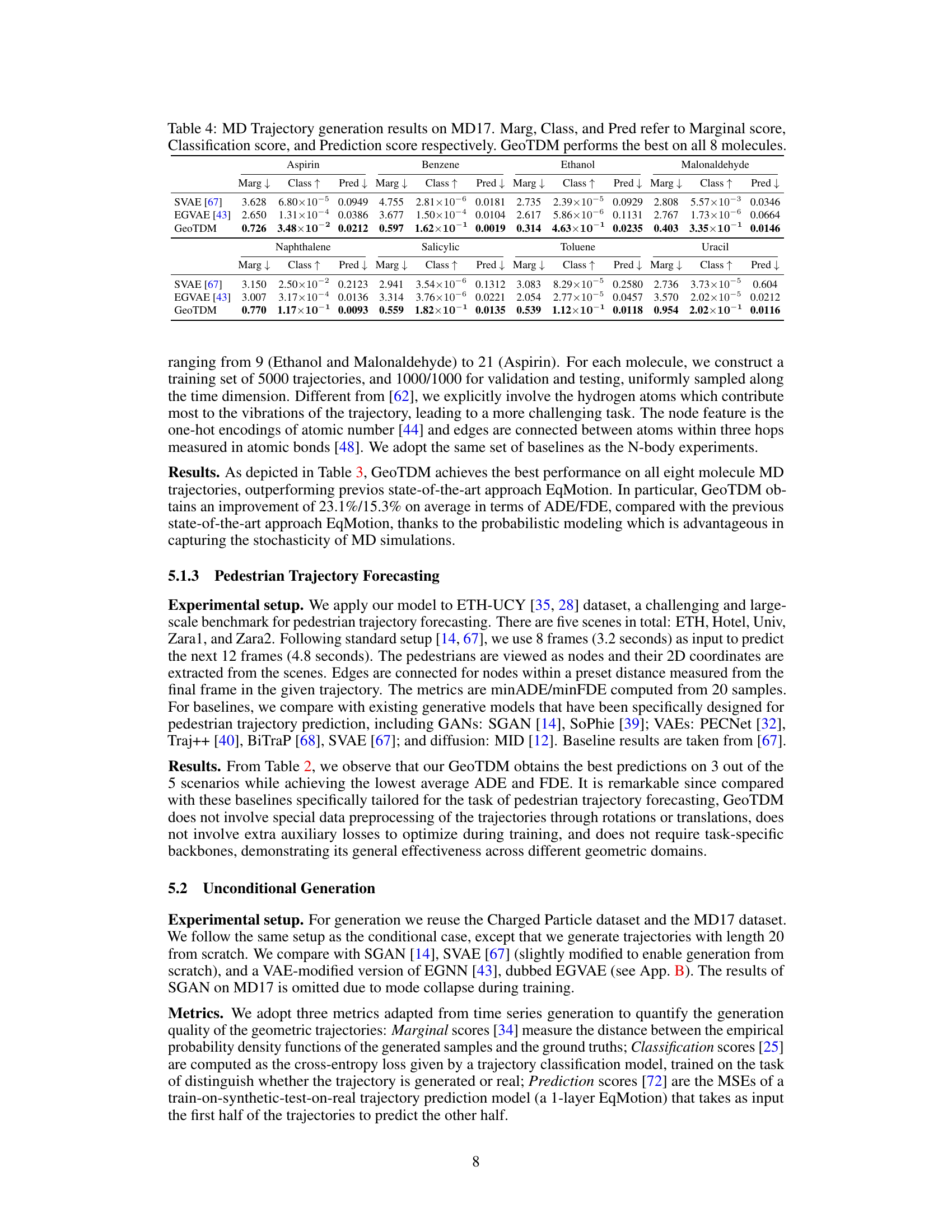
🔼 This table presents the results of conditional trajectory generation experiments on the MD17 dataset. The dataset consists of molecular dynamics trajectories of small molecules. The table shows the Average Displacement Error (ADE) and Final Displacement Error (FDE) for different trajectory generation methods. The methods are compared across multiple molecules, allowing for an evaluation of their performance in diverse scenarios. Lower ADE and FDE values indicate better performance.
read the caption
Table 3: Conditional trajectory generation on MD17. Results averaged over 5 runs (std in App. C.4).

🔼 This table presents the results of MD trajectory generation on the MD17 dataset using various models including SVAE, EGVAE, and the proposed GeoTDM. The performance of each model is evaluated using three metrics: Marginal score (Marg↓), Classification score (Class ↑), and Prediction score (Pred↓). Lower scores indicate better performance for Marg and Pred, while a higher score is better for Class. The table shows that GeoTDM achieves the best performance across all eight molecules in the dataset.
read the caption
Table 4: MD Trajectory generation results on MD17. Marg, Class, and Pred refer to Marginal score, Classification score, and Prediction score respectively. GeoTDM performs the best on all 8 molecules.
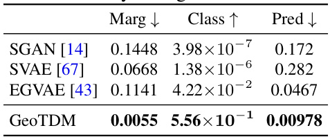
🔼 This table presents a comparison of unconditional generation results on the N-body Charged Particle dataset. It compares the performance of GeoTDM against three baselines (SGAN, SVAE, and EGVAE) across three metrics: Marginal score (lower is better), Classification score (higher is better), and Prediction score (lower is better). The Marginal score quantifies the difference between the generated samples’ empirical probability density and that of the ground truth. The Classification score assesses the model’s ability to generate samples indistinguishable from the real data. The Prediction score evaluates a prediction model’s accuracy when trained on synthetic data and tested on real data, measuring how well the generated samples can mimic real-world patterns.
read the caption
Table 5: Unconditional generation results on N-body Charged Particle.
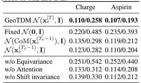
🔼 This table presents the ablation study results for the GeoTDM model. It shows the impact of different design choices on the model’s performance, measured by ADE and FDE. Specifically, it compares the performance of GeoTDM with several variants: using a fixed Gaussian prior (N(0,I)), using a CoM-based prior (N(COM(xTc-1c),I)), using a point-wise prior (N(xTc-1c,I)), removing equivariance, removing attention, and removing shift invariance. The results are presented for the Charged Particle and Aspirin datasets.
read the caption
Table 6: Ablation studies. The numbers refer to ADE/FDE.

🔼 This table lists the hyperparameters used for training the GeoTDM model on three different datasets: N-body, MD, and ETH. For each dataset, it shows the number of layers in the EGTN, the hidden dimension of the network, the dimension of the temporal embedding, the number of timesteps (T) in the trajectory, the batch size, and the learning rate used during training. These hyperparameters were chosen to optimize performance on each respective task.
read the caption
Table 7: Hyper-parameters of GeoTDM in the experiments.

🔼 This table presents the results of experiments conducted to evaluate the impact of varying the number of diffusion steps (T) on the performance of the GeoTDM model. The upper half shows results for unconditional generation, while the lower half shows results for conditional forecasting. Metrics reported include Marginal score (lower is better), Classification score (higher is better), and Prediction score (lower is better) for the unconditional generation. For conditional forecasting, the metrics reported are ADE (Average Displacement Error), FDE (Final Displacement Error), and NLL (Negative Log Likelihood) (lower is better for all). The results demonstrate the trade-off between the number of diffusion steps and model performance. Increasing T generally improves performance, but at the cost of increased computational resources.
read the caption
Table 8: The effect of diffusion steps in the unconditional generation setting (top) and conditional forecasting setting (bottom).

🔼 This table compares the sampling runtime and generation metrics of GeoTDM with different numbers of diffusion steps (100 and 1000) against EGVAE, an autoregressive VAE-based model. It demonstrates the trade-off between sampling speed and the quality of the generated samples. While GeoTDM is slower due to the iterative nature of diffusion models, it achieves significantly better generation quality.
read the caption
Table 9: Sampling runtime comparison on MD17 Aspirin molecule.

🔼 This table shows the results of conditional trajectory generation on three different N-body simulation datasets: charged particles, spring dynamics, and gravity. The performance of GeoTDM is compared against the SVAE baseline, using Average Displacement Error (ADE) and Final Displacement Error (FDE) as metrics. The results are averaged over 5 runs, and standard deviations are reported.
read the caption
Table 10: Conditional generation results of GeoTDM on N-body charged particle, spring, and gravity. Results (mean ± standard deviation) are computed from 5 samples.

🔼 This table presents the results of conditional trajectory generation on the MD17 dataset using the GeoTDM model. It shows the Average Displacement Error (ADE) and Final Displacement Error (FDE) for eight different small molecules: Aspirin, Benzene, Ethanol, Malonaldehyde, Naphthalene, Salicylic acid, Toluene, and Uracil. The values are the means and standard deviations calculated across five runs for each molecule.
read the caption
Table 11: Conditional generation results of GeoTDM on MD17. Results (mean ± standard deviation) are computed from 5 samples.

🔼 This table summarizes the key differences between GeoTDM and existing methods for geometric trajectory modeling, highlighting whether each method handles trajectories, incorporates equivariance, supports conditional and unconditional generation, and utilizes a learnable prior. It provides a concise comparison of capabilities.
read the caption
Table 12: Technical differences between GeoTDM and existing works.
Full paper#

