↗ OpenReview ↗ NeurIPS Homepage ↗ Chat
TL;DR#
Understanding how deep neural networks (DNNs) make decisions is a major challenge in AI research. Current methods for evaluating the interpretability of individual units within DNNs rely heavily on time-consuming and expensive human evaluation, limiting the scope of research. This hinders the development of more interpretable and trustworthy AI systems.
This research paper tackles this issue by proposing a novel, fully automated method for measuring per-unit interpretability in vision DNNs. The method uses an advanced image similarity function and a binary classification task, eliminating the need for human judgment. The researchers validate their method through extensive experiments, including an interventional psychophysics study. They reveal interesting relationships between interpretability and various factors such as model architecture, layer properties and training dynamics.
Key Takeaways#
Why does it matter?#
This paper is crucial for AI researchers as it introduces the first scalable and human-free method for measuring per-unit interpretability in vision DNNs. This breakthrough removes the bottleneck of human evaluation, enabling large-scale analyses previously infeasible. The findings challenge existing assumptions about the relationship between model performance and interpretability, opening exciting new avenues for research in model design and optimization.
Visual Insights#

This figure illustrates the method used to create a machine interpretability score (MIS). Panel A shows the established human psychophysics task to measure per-unit interpretability in a neural network. The task requires participants to match query images (strongly activating the unit) with visual explanations (also strongly activating the unit). Panel B describes the automated version replacing humans, using a feature encoder (DreamSim) and a classifier to predict the probability of a correct match across multiple tasks. The MIS is the average predicted probability. Panel C demonstrates that the automated MIS strongly correlates with human interpretability ratings.

This table shows the sensitivity analysis of the sparsity and machine interpretability score (MIS) of Sparse Auto-encoders (SAEs) in relation to the hyperparameters. It demonstrates how different sparsity weight values affect the number of non-zero elements (LO Count) and the resulting MIS values.
In-depth insights#
Scale Auto Intrp#
The heading ‘Scale Auto Intrp,’ likely short for “Scalable Automated Interpretability,” points towards a crucial advancement in the field of Explainable AI (XAI). The core idea revolves around developing methods to automatically assess the interpretability of individual units (neurons or channels) within large neural networks, thus overcoming the limitations of manual human evaluation. This automation is key to scaling interpretability analysis to the massive models prevalent today. The approach would likely involve designing a robust metric that correlates well with human judgments of interpretability. This metric would then be applied to millions, even billions, of units across numerous models to identify patterns and trends in how these units process information and contribute to overall model performance. A successful “Scale Auto Intrp” methodology would unlock large-scale, high-throughput experimentation, facilitating new research on model architecture design, training strategies, and the inherent mechanisms of information processing within deep learning models. Such an advance would significantly improve our understanding of deep learning’s inner workings and potentially pave the way for the creation of more reliable, efficient, and interpretable AI systems. However, challenges remain; the accuracy of the automated metric in reflecting human perception is paramount and would require extensive validation. Additionally, dealing with the computational demands of such large-scale analysis needs careful consideration.
MIS Validation#
The MIS validation section is crucial for establishing the reliability and predictive power of the proposed Machine Interpretability Score. It likely involves comparing the MIS against existing human interpretability annotations, possibly using established metrics like correlation coefficients. Strong positive correlations would be highly desirable, demonstrating that the automated MIS accurately reflects human judgments of unit interpretability. The validation likely includes rigorous statistical testing to ensure the significance of the findings. Ideally, the paper would detail the dataset used for validation, specifying its size, the diversity of models it encompasses, and the methods used for collecting human judgments. Investigating the MIS’s performance across various model architectures and explanation methods is also essential. Exploring limitations or edge cases where the MIS might underperform human evaluations is critical for transparently assessing its generalizability and robustness. Ultimately, a robust validation establishes the MIS as a reliable, scalable alternative to manual human evaluation for measuring the interpretability of deep learning models.
Layer Effects#
Analyzing layer effects in deep neural networks is crucial for understanding their internal workings. Depth often shows an initial increase in interpretability, possibly due to simpler features being learned in early layers. However, interpretability can decrease in later layers as the network learns more complex, abstract representations. Width may also significantly affect interpretability. Wider layers, with more units, could potentially lead to increased interpretability, possibly due to a greater capacity for disentangling features. Layer type also impacts interpretability; convolutional layers might generally show higher interpretability than normalization or linear layers, reflecting their role in feature extraction. These layer effects interplay in complex ways; changes in depth can cause varying effects on interpretability across layers with different widths and types, requiring more investigation into these interactions.
Training Dynamics#
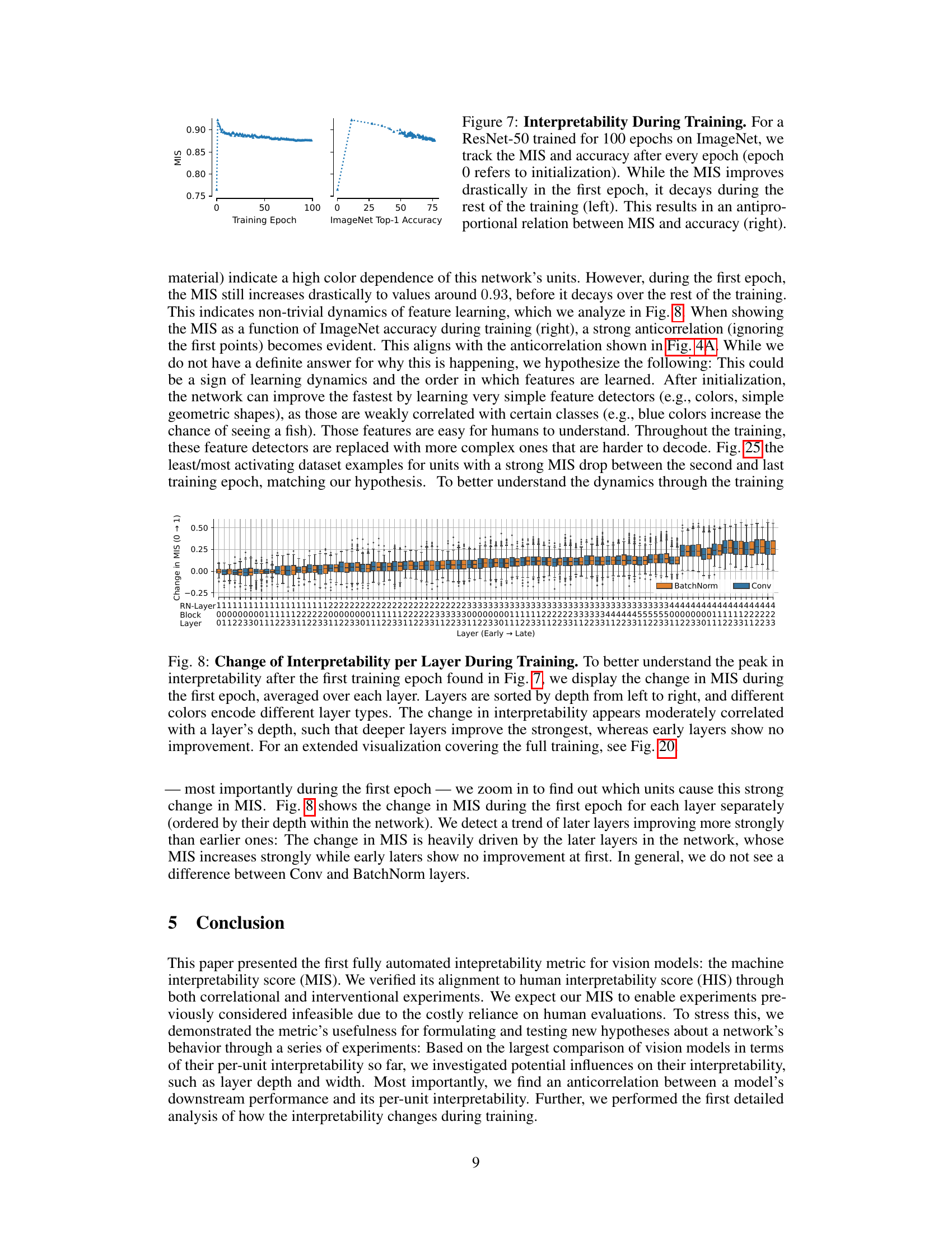
Analyzing the training dynamics of deep neural networks is crucial for understanding their learning mechanisms. The paper investigates how the Machine Interpretability Score (MIS), a novel automated measure of interpretability, changes during the training process. The initial MIS is already above chance level, suggesting that the network even in its untrained state possesses some degree of inherent interpretability. A significant increase in MIS is observed during the first epoch, which indicates that the network rapidly learns simple, easily understandable features at the beginning of training. Subsequently, the MIS gradually declines during the remaining training epochs. This counterintuitive finding suggests that the network transitions from learning simple features to more complex, less interpretable representations as training progresses. This observation aligns with the general trend in deep learning, where initial progress tends to be faster and more intuitive, while later stages involve the learning of subtle interactions that are less readily explainable. The anticorrelation observed between MIS and accuracy highlights the trade-off between interpretability and performance in deep neural networks. Understanding this dynamic is critical for designing more interpretable models without sacrificing accuracy.
Future XAI#
Future XAI research should prioritize developing more robust and scalable methods for evaluating interpretability. Current approaches often rely on human judgments, limiting their applicability to large-scale analyses. Automated metrics that accurately reflect human perception are crucial. Causality needs further exploration; while correlation between model features and outputs is valuable, understanding the true causal relationships is vital for trust and reliability. The development of interpretable-by-design models should be a focus, shifting from post-hoc explanations to building inherent transparency into AI systems. Benchmarking and standardization of interpretability methods are essential to ensure fair comparisons and facilitate progress. Finally, research should address ethical concerns, ensuring that future XAI techniques are fair, equitable, and mitigate potential biases.
More visual insights#
More on figures

This figure validates the Machine Interpretability Score (MIS) by comparing it to existing human interpretability scores (HIS). Panel A shows that MIS accurately reproduces the model ranking from the IMI dataset, demonstrating its ability to predict model-level interpretability without human evaluation. Panel B shows a strong correlation between MIS and HIS at the unit level, indicating that MIS effectively predicts unit-level interpretability as well. Panel C further validates MIS by showing that units selected as ‘hardest’ (lowest MIS) and ’easiest’ (highest MIS) by MIS indeed demonstrate significantly lower and higher interpretability, respectively, in a human psychophysics study compared to random units.

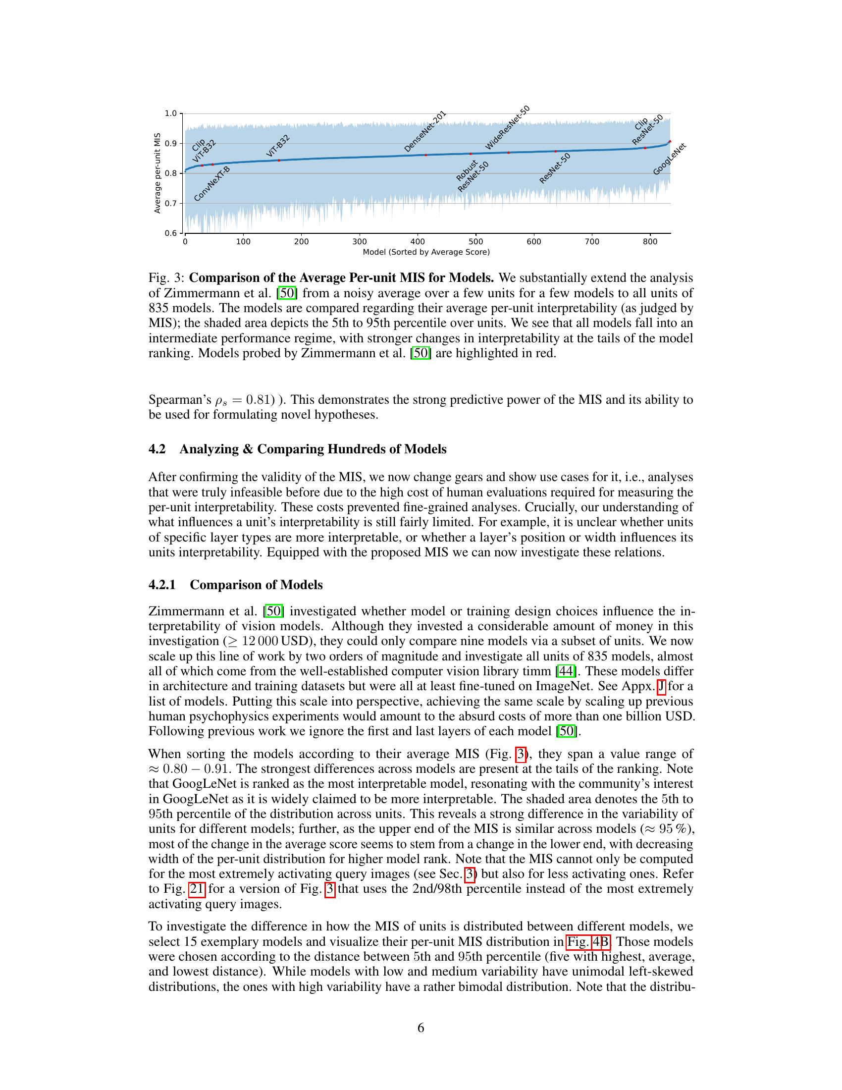
This figure displays the average per-unit machine interpretability score (MIS) for 835 different vision models. The models are ranked by their average MIS. The shaded region shows the 5th to 95th percentile range of MIS values across all units within each model, highlighting the variability in interpretability among units within a single model. The figure demonstrates a substantial increase in the scale of the interpretability analysis compared to previous work, showing the average interpretability for a substantially larger number of models and units.

This figure shows the relationship between ImageNet accuracy and the average per-unit Machine Interpretability Score (MIS) across 835 models. Panel A displays a scatter plot showing a negative correlation between ImageNet top-1 accuracy and the average per-unit MIS. Panel B presents kernel density estimations of the per-unit MIS distribution for 15 models selected to represent the range of variability observed in the data. Models with low variability exhibit a unimodal distribution, while models with high variability display a bimodal distribution, indicating the presence of both highly and lowly interpretable units within those models.

This figure compares the average per-unit Machine Interpretability Score (MIS) across 835 different computer vision models. The x-axis represents the models sorted by their average MIS, and the y-axis shows the average per-unit MIS. The shaded area represents the 5th to 95th percentile range of MIS values across all units within each model. The authors highlight models previously analyzed in Zimmermann et al. [50] in red. The figure demonstrates a substantial extension of prior work, evaluating per-unit interpretability on a larger scale. It shows that the models cluster within a medium range of interpretability, with more variation at the extremes of model ranking. This suggests that model architecture and training significantly impact interpretability.

This figure analyzes the relationship between a layer’s position and width within a neural network and its interpretability, as measured by the Machine Interpretability Score (MIS). Panel (A) shows that deeper layers tend to be more interpretable, exhibiting an almost sinusoidal relationship with relative depth. Panel (B) indicates a positive correlation between a layer’s width and its interpretability, although this effect is weaker for batch normalization layers.

This figure shows the training dynamics of a ResNet-50 model on ImageNet. The left panel plots the Machine Interpretability Score (MIS) against training epoch, illustrating a sharp increase in MIS during the first epoch, followed by a gradual decline throughout the remaining training process. The right panel depicts the relationship between MIS and ImageNet Top-1 accuracy, revealing an inverse correlation between the two metrics after the initial epoch. This suggests a trade-off between model interpretability and performance during training.

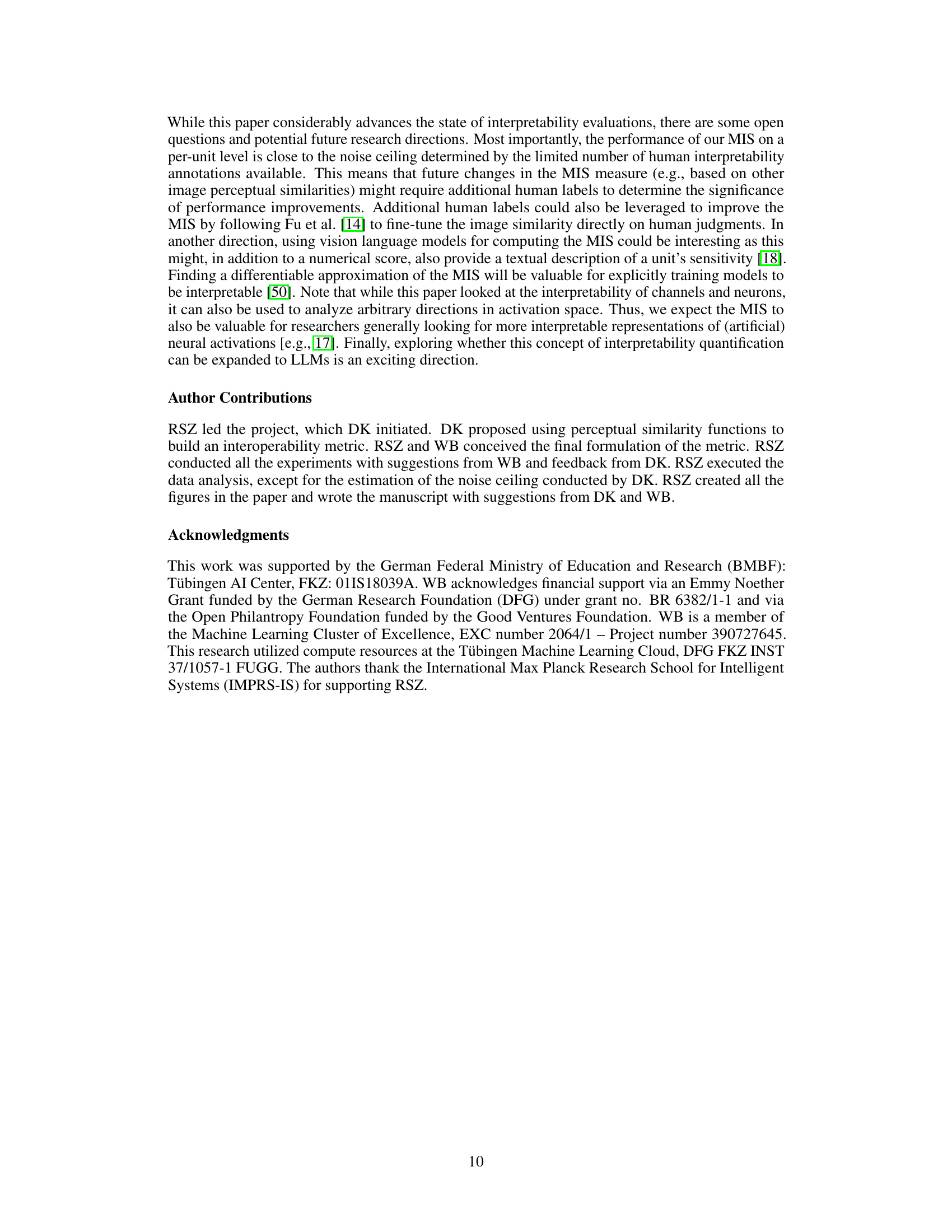
This figure shows how the average per-unit Machine Interpretability Score (MIS) changes for each layer during the first training epoch. The change in MIS is plotted against the layer’s relative depth within the network (from early layers to late layers). Different colors represent different layer types. The results reveal a moderate correlation between the change in interpretability and layer depth, with deeper layers showing greater improvement than earlier layers. A more detailed visualization of the change in MIS throughout the entire training process is available in Figure 20.

This figure shows two examples of the 2-Alternative Forced Choice (2-AFC) task used in the paper. The task is designed to measure how well a participant understands the sensitivity of a unit in a neural network. Each task consists of: 1. Negative Explanations: Images that minimally activate the unit. 2. Positive Explanations: Images that maximally activate the unit. 3. Queries: Two query images, one of which strongly activates the unit and one which weakly activates the unit. The participant’s job is to select which of the query images corresponds to the positive explanations, demonstrating their understanding of the unit’s activation patterns.

This figure describes the Machine Interpretability Score (MIS) which is a fully automated method to quantify per-unit interpretability. Panel A shows the established task definition for human psychophysics experiments to measure per-unit interpretability. Panel B shows how the proposed method automates this evaluation. Instead of humans, it uses a feature encoder and a binary classifier. The MIS is the average of the predicted probability of a correct choice over several tasks. Panel C illustrates that the MIS correlates well with human interpretability ratings.
This figure validates the Machine Interpretability Score (MIS) by comparing it to existing Human Interpretability Scores (HIS). Panel A shows that the MIS accurately reproduces the model ranking from a previous study, demonstrating its ability to predict model-level interpretability without human input. Panel B shows a strong correlation between MIS and HIS at the unit level, indicating that the MIS can also accurately predict the interpretability of individual units. Finally, Panel C demonstrates the predictive power of the MIS by showing that units with high MIS scores are significantly more interpretable than randomly selected units, while units with low MIS scores are significantly less interpretable, thereby demonstrating the method’s predictive power in a causal intervention.

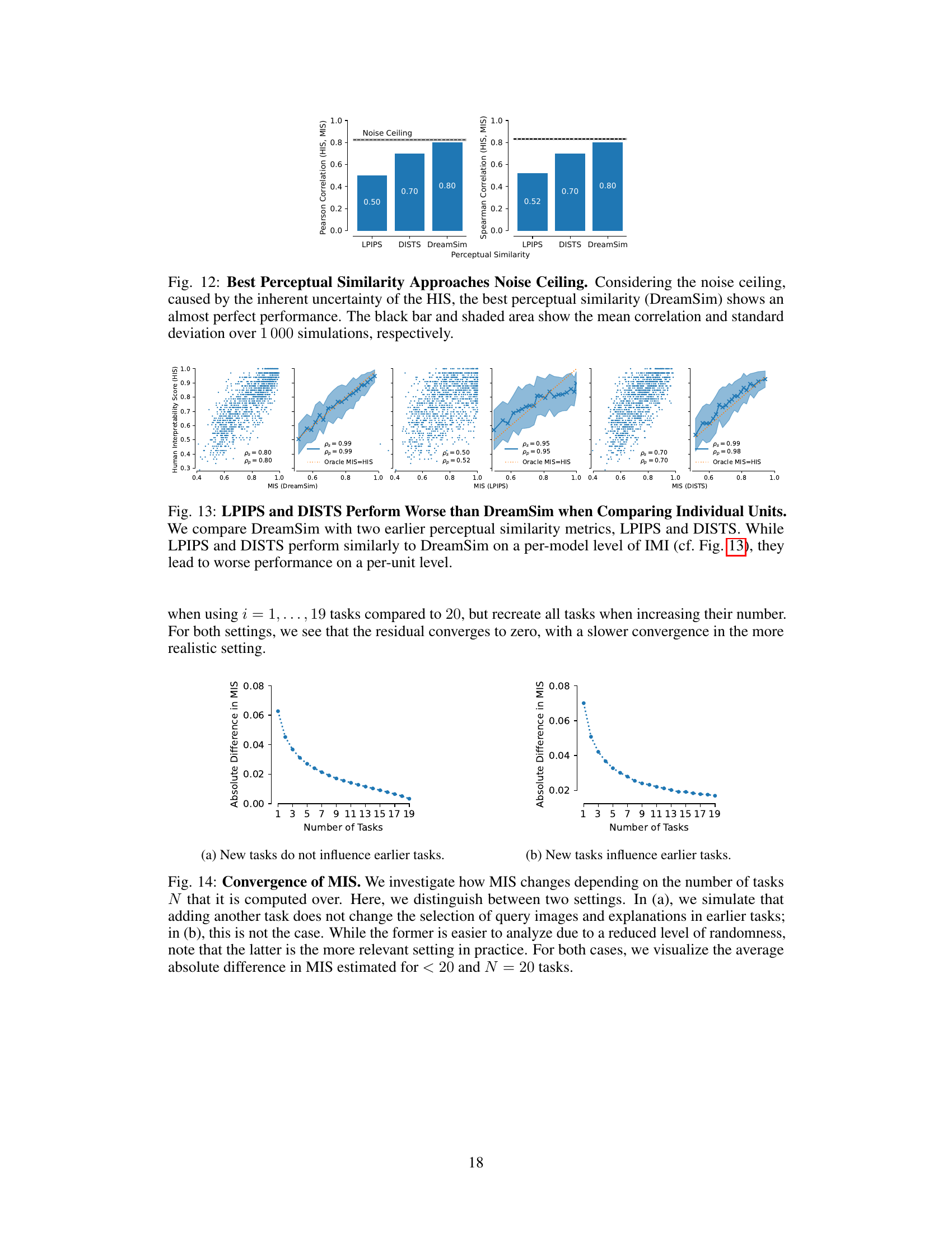
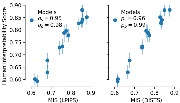
This figure compares three different perceptual similarity measures (LPIPS, DISTS, and DreamSim) used in calculating the Machine Interpretability Score (MIS). It shows that DreamSim outperforms the others in terms of correlation with Human Interpretability Score (HIS), even when considering the noise ceiling (the theoretical maximum correlation due to limitations in human annotation). The noise ceiling is represented by the dashed horizontal line, and the bars show the average correlation with HIS along with the standard deviation over 1000 simulations.

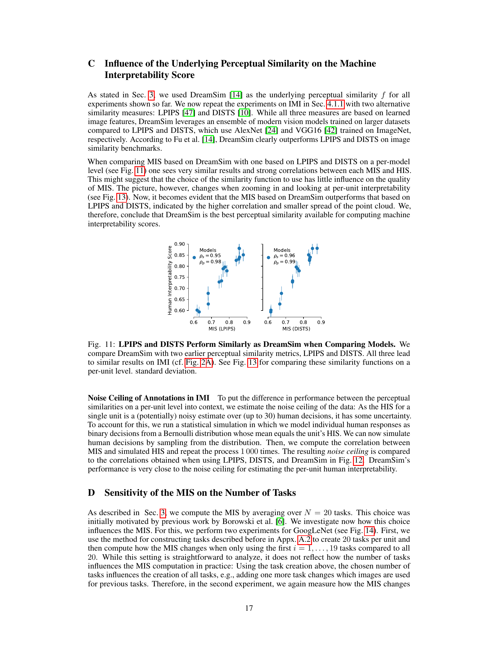
This figure compares the performance of three different perceptual similarity metrics (DreamSim, LPIPS, and DISTS) when used to compute the Machine Interpretability Score (MIS). The metrics are evaluated based on how well the resulting MIS correlates with human interpretability scores from the IMI dataset. The results show that DreamSim and LPIPS achieve similar overall results when comparing models, but DreamSim performs better at a finer-grained, per-unit level, as shown in a subsequent figure (Figure 13).
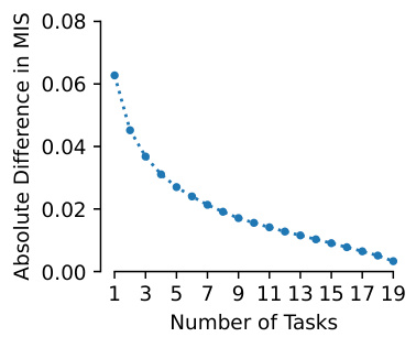
This figure analyzes the impact of the number of tasks (N) used to calculate the Machine Interpretability Score (MIS) on its stability. Two scenarios are compared: one where adding tasks does not affect previously selected image-explanation pairs, and a more realistic scenario where adding new tasks influences the selection of all pairs. The plots show the average absolute difference in MIS when using fewer than 20 tasks compared to using all 20 tasks. The results indicate a convergence towards zero as the number of tasks increases, demonstrating the stability and reliability of the MIS estimation with sufficiently many tasks.
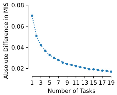
This figure shows how the Machine Interpretability Score (MIS) changes depending on the number of tasks used to compute it. Two scenarios are considered: one where adding a task doesn’t affect previous tasks, and another where it does. The graph plots the average absolute difference in MIS between using fewer tasks (1 to 19) and using the full 20 tasks. The results show that the MIS converges to a stable value as more tasks are used, with convergence being slower in the more realistic scenario (where new tasks influence the selection of previous tasks).
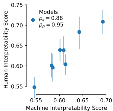
This figure validates the Machine Interpretability Score (MIS) by comparing it to existing human interpretability annotations (HIS). Panel A shows that MIS accurately reproduces model rankings from the IMI dataset, demonstrating its ability to predict model-level interpretability without human evaluation. Panel B demonstrates that MIS also predicts per-unit interpretability, showing a strong correlation with HIS. Panel C further validates MIS by conducting a causal intervention study, where the easiest and hardest interpretable units identified by MIS are confirmed through a psychophysics experiment, highlighting the measure’s predictive power.

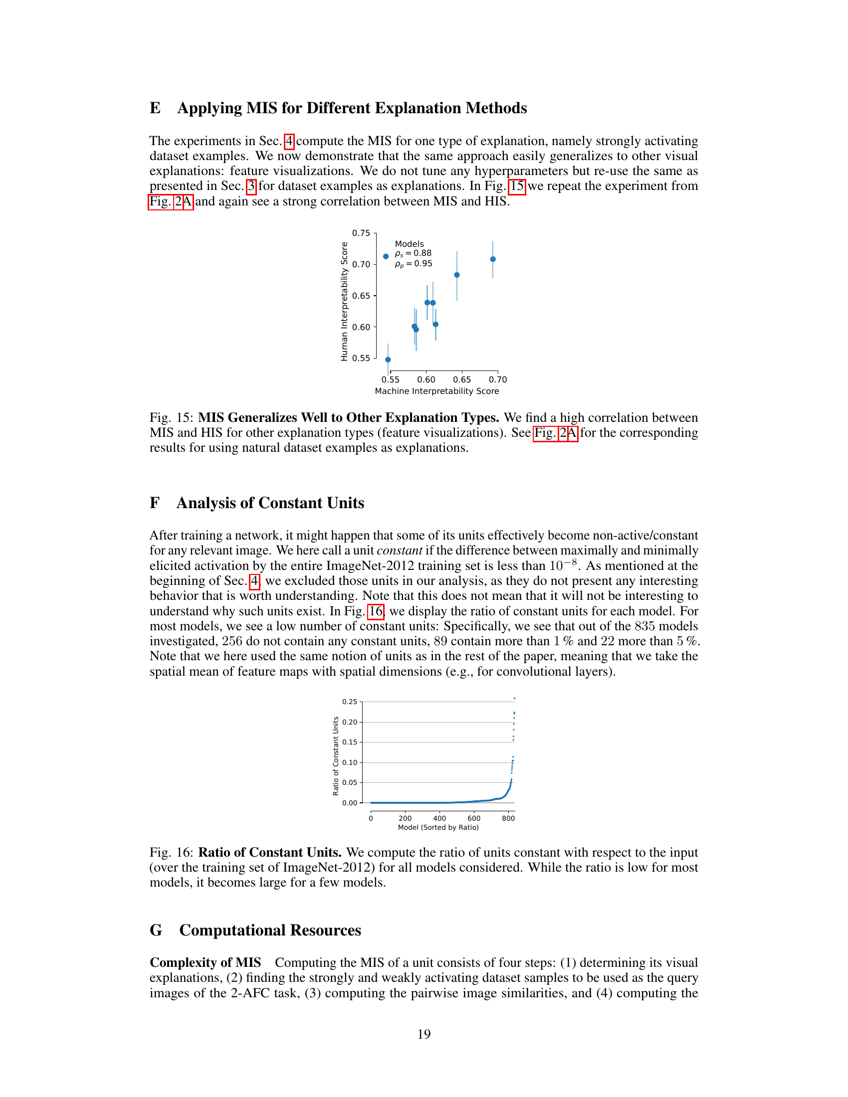
This figure shows the ratio of constant units for each of the 835 models investigated in the paper. A unit is considered constant if the difference between its maximum and minimum activation across all images in the ImageNet-2012 training set is less than 10⁻⁸. The x-axis represents the models sorted by the ratio of constant units, and the y-axis shows that ratio. The majority of models have a low ratio of constant units, but some models exhibit a significantly higher ratio. This indicates the prevalence of inactive or constant units in a subset of the analyzed models.

This figure compares the performance of two different types of sparse autoencoders (SAEs) in terms of their sparsity, reconstruction fidelity, and interpretability, using the Machine Interpretability Score (MIS) as a metric. It shows that while Gated SAEs offer a better balance between sparsity and reconstruction fidelity, both types achieve a similar level of interpretability as measured by MIS. Notably, the SAEs’ interpretability remains comparable to the original layer’s interpretability, despite exhibiting higher sparsity.

This figure shows the statistical significance of the differences between different layer types’ MIS. The results are from a Conover’s test that compares per-model and per-layer-type MIS means, with Holm’s correction applied for multiple comparisons. The heatmap displays the significance levels (p-values) for each pairwise comparison between layer types. Darker colors indicate stronger statistical significance.
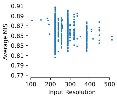
This figure shows the relationship between ImageNet accuracy and the Machine Interpretability Score (MIS). Panel A demonstrates a negative correlation: higher accuracy models tend to have lower average per-unit MIS. Panel B displays the distribution of per-unit MIS across 15 models, categorized by variability. Models with low variability show unimodal distributions, whereas those with high variability exhibit bimodal distributions, indicating a subset of less interpretable units.
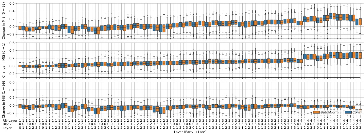
This figure provides a more detailed visualization of the change in the machine interpretability score (MIS) during the training process of a ResNet-50 model on ImageNet-2012. It expands on Figure 8 by showing the change in MIS for each layer across all training epochs. The graph displays how the interpretability of different layer types (BatchNorm and Conv) changes over time, providing a more nuanced understanding of the learning dynamics and feature evolution within the network. This detailed layer-by-layer breakdown gives insight into how different layer types contribute to overall model interpretability during training.

This figure shows the average per-unit machine interpretability score (MIS) for 835 different models. The x-axis represents the models sorted by their average MIS. The y-axis shows the average per-unit MIS. The shaded area indicates the 5th to 95th percentile range of MIS across units within each model. The figure highlights that while there is a range in average interpretability across models, most models fall within a similar range. The models tested in previous work by Zimmermann et al. [50] are marked in red for comparison.

This figure shows the average per-unit Machine Interpretability Score (MIS) for 835 different models. The models are ranked by their average MIS, which is a measure of how easily humans can understand the units (e.g. neurons or channels) in a vision model. The shaded region shows the 5th to 95th percentile of MIS across all units within each model, illustrating the variability in interpretability among units within the same model. The figure demonstrates that even though model rankings by interpretability correlates well with previous results using much smaller datasets, it also presents novel information on the wide variability of units’ interpretability within a model.

This figure shows the relationship between the average per-unit machine interpretability score (MIS) and layer depth and width. Panel A displays the average MIS for different layer types (convolutional, linear, batchnorm, layernorm, groupnorm) as a function of relative layer depth. A sinusoidal pattern is observed across layer types, with an initial increase, a dip in the middle, and a final drop towards the end of the network. Panel B presents a similar analysis but focuses on layer width and shows a relatively consistent and slight increase in MIS across different layer types with an increase in relative layer width. This visualization indicates that deeper and wider layers tend to have higher interpretability scores.

This figure shows the relationship between the average per-unit machine interpretability score (MIS) and the relative layer depth/width for different layer types. Panel (A) demonstrates that deeper layers generally have a higher average MIS. Panel (B) shows that wider layers also tend to have higher average MIS. This suggests a correlation between layer depth/width and model interpretability.
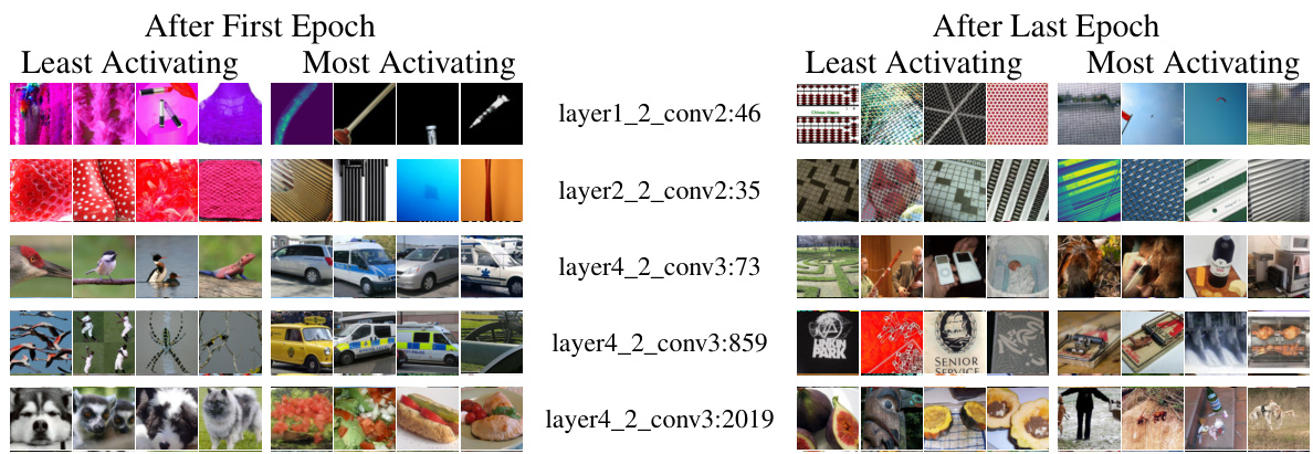
This figure shows the least and most activating dataset examples for four units of a ResNet50 model. The left column displays examples from after the first training epoch, and the right column displays examples from after the last epoch. The caption highlights that while the units initially respond strongly to easily understandable visual features (e.g., color), later in training they respond to more complex and less interpretable features, resulting in a decrease in their Machine Interpretability Score (MIS). The units shown are those that experience the most significant drop in MIS during training.

This figure shows four examples of units where the Machine Interpretability Score (MIS) overestimates the Human Interpretability Score (HIS). Each unit’s 20 most and 20 least activating images (visual explanations) are displayed. The goal is to illustrate instances where the automated MIS metric doesn’t perfectly align with human perception of interpretability.

This figure shows two examples of the 2-AFC (two-alternative forced choice) task used to evaluate the interpretability of units in a deep neural network. Each example shows two sets of images (positive and negative explanations) that represent the patterns a unit responds to strongly and weakly, respectively. Two additional query images are presented, and the task is to determine which query image matches the positive explanations better. This task assesses human understanding of a unit’s sensitivity by requiring participants to match strongly activating images to the strongly activating visual explanations.

This figure shows two examples of the two-alternative forced-choice (2-AFC) task used in the paper to measure per-unit interpretability. Each example displays sets of positive and negative visual explanations (images that strongly activate or deactivate the unit in question) alongside two query images. The task is to determine which query image best matches the positive explanations. This task is used to evaluate how well participants (either humans or a machine in the automated version) understand the sensitivity of a unit by assessing their ability to match strongly activating query images with strongly activating visual explanations.
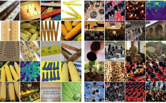
This figure shows two examples of the 2-AFC (two-alternative forced choice) task used to measure per-unit interpretability. Each task consists of three parts: (1) Negative explanations (minimally activating images for the unit), (2) Positive explanations (maximally activating images), and (3) Two query images (test images). The participant is asked to choose which query image better matches the positive explanations.
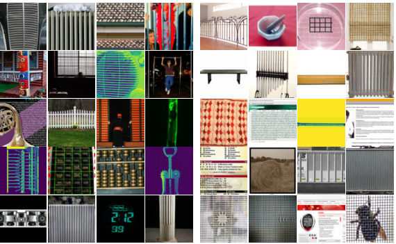
This figure shows two examples of the two-alternative forced-choice (2-AFC) task used in the paper to evaluate the interpretability of units in a neural network. Each task presents participants with two query images (center) and two sets of visual explanations: one set showing images that strongly activate the unit (positive explanations, right), and one set showing images that minimally activate the unit (negative explanations, left). Participants must choose which of the two query images better matches the positive explanations.

This figure shows two examples of the 2-alternative forced choice (2-AFC) task used to evaluate per-unit interpretability. Each example shows two sets of images: positive explanations (maximally activating images for a specific unit in a neural network) and negative explanations (minimally activating images). In the center are two query images, one which strongly and one which weakly activates the unit. The task is for the participant (or the machine in the automated version) to determine which query image is the positive example (i.e., matches the positive explanations).

This figure shows two examples of the two-alternative forced-choice (2-AFC) task used in the paper to evaluate unit interpretability. Each example shows sets of positive and negative visual explanations (images) for a specific unit in a GoogLeNet model. The positive explanations are images that maximally activate the unit, while the negative explanations are images that minimally activate it. Two query images (test images) are presented, and the task is for the participant (human or machine) to select the query image that best matches the positive explanations based on their perceived similarity.
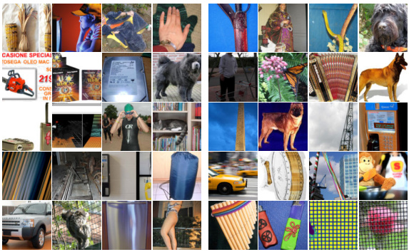
This figure shows two examples of the two-alternative forced-choice (2-AFC) task used to evaluate the per-unit interpretability of units in deep neural networks. In each example, there are sets of ‘positive’ and ’negative’ visual explanations (images representing strongly and weakly activating inputs to the unit, respectively) presented to the user alongside two query images. The task is to select the query image that best corresponds to the positive explanations. The figure highlights the challenge in determining which of the query images is the correct answer for the human participants in the original study, and how this task is automated using machine learning methods in the paper.
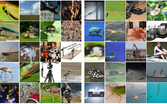
This figure shows two examples of the 2-AFC (two-alternative forced-choice) task used to evaluate the per-unit interpretability of units in a convolutional neural network (CNN). The task presents participants with two query images and two sets of visual explanations (positive and negative). The positive examples illustrate the patterns that maximally activate the unit. Conversely, the negative examples show patterns that minimally activate the unit. The goal is for participants to determine which query image corresponds to the positive explanations (i.e., which image elicits higher unit activation). The figure highlights the importance of using both query images and explanations to assess a unit’s sensitivity.
Full paper#
