TL;DR#
Transformer models are increasingly used in deep learning, but their optimization stability and behavior as their size increases remain a challenge. One approach is to find parameterizations that give scale-independent feature updates, enabling stable and predictable scaling. This paper focuses on randomly initialized transformers and investigates various scaling limits during training.
This research uses dynamical mean field theory (DMFT) to study these infinite limits. By analyzing different scaling approaches, they identify specific parameterizations that allow attention layers to update effectively during training. The findings reveal how different infinite limits lead to unique statistical descriptions, depending on how the attention layers are scaled. This directly informs the optimal strategy for scaling up transformer models for better performance.
Key Takeaways#
Why does it matter?#
This paper is crucial because it offers a theoretical framework for understanding the scaling behavior of transformer models, a critical aspect for improving their performance and efficiency. It also provides practical guidance for parameterizing these models to optimize training and feature learning, directly impacting large-scale AI development.
Visual Insights#

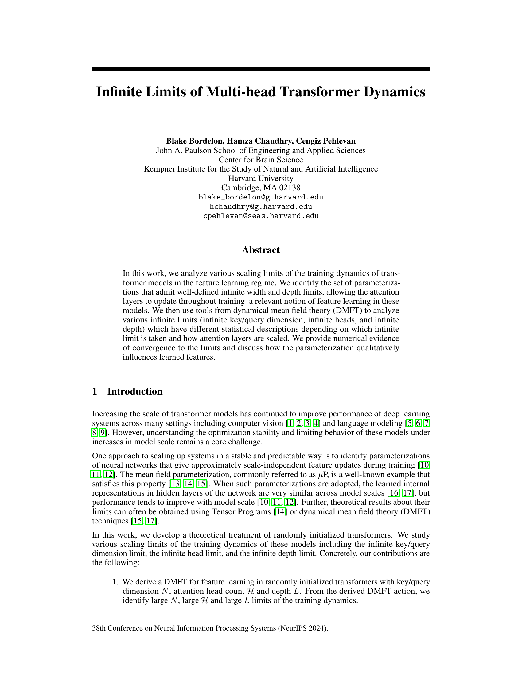
🔼 This figure schematically shows the architecture of the transformer model used in the paper. Panel (a) illustrates the forward pass through the residual stream, highlighting the alternating MHSA and MLP blocks, which are scaled by the factor βoL-αι (βo: constant, L: depth, αL: scaling exponent). Panel (b) details the MHSA block, which computes keys, queries, values, and attention variables to generate a concatenated output with a dimension of dmodel = NH (N: key/query dimension, H: number of heads).
read the caption
Figure 1: Schematic representations of the transformer architecture we model. (a) The forward pass through the residual stream is an alternation of MHSA and MLP blocks scaled by βoL-αι. (b) The MHSA block computes keys, queries, values, and attention variables to produce a concatenated output of dimension dmodel = NH.

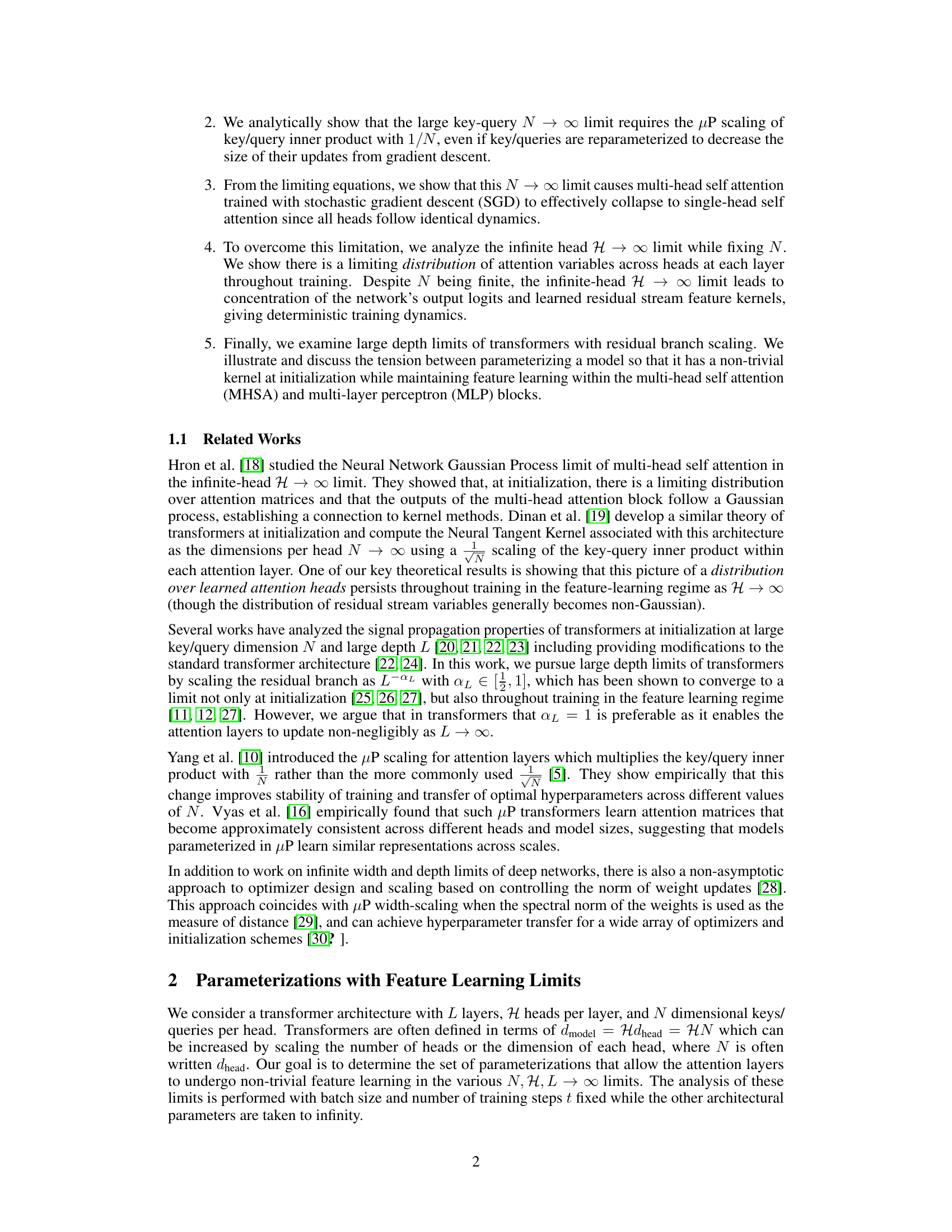
🔼 This table shows how to scale the learning rate for both SGD and Adam optimizers to maintain the correct scale of updates to the weights and variables when using the parameterizations described in the paper. It also indicates how the variance and multipliers for the first layer should be rescaled, depending on the chosen optimizer and parameterization.
read the caption
Table 1: The learning rates which should be applied to obtain the correct scale of updates for SGD or Adam optimizers. In addition, the weight variance and multiplier for the first layer may need to be rescaled (relative to eq (5)) with width/depth depending on the parameterization and optimizer.
In-depth insights#
Infinite Limits#
The concept of ‘Infinite Limits’ in the context of a research paper likely refers to the mathematical analysis of model behavior as specific parameters tend towards infinity. This is a common technique in studying the theoretical properties of large-scale neural networks, such as transformers. The study of infinite limits helps to understand the fundamental characteristics of these models, moving beyond empirical observations and towards a more principled understanding of their capabilities and limitations. This often involves using tools from statistical physics, such as dynamical mean field theory (DMFT), to derive simplified equations describing the system’s behavior under extreme conditions. Examining these limits reveals important insights, including whether models learn consistent features across different scales and how the choice of parameterizations influences the model’s dynamics and capacity for learning. A key benefit is that it can assist in designing stable and predictable scaling strategies for building larger and more powerful models.
DMFT Analysis#
The DMFT (Dynamical Mean Field Theory) analysis section of the research paper is crucial for understanding the complex training dynamics of transformer models. DMFT provides a theoretical framework to analyze the infinite-width or infinite-depth limits of neural networks, offering insights not readily available through empirical methods alone. The authors likely used DMFT to derive equations describing the evolution of relevant quantities such as feature kernels, gradient kernels, and attention matrices throughout the training process. This mathematical analysis allows for a deeper understanding of the model’s behavior in various scaling regimes, illuminating how the training dynamics are affected by changes in key parameters like the number of heads, the dimension per head, and the depth of the network. The results would likely provide valuable insights into the stability, efficiency, and generalization capacity of large transformer models. By identifying the parameterizations that admit well-defined infinite limits, the study sheds light on how model design choices can impact the learned internal representations. Further, the DMFT approach would likely highlight the relationship between the learned features and the optimization dynamics, revealing how certain architectural choices facilitate efficient feature learning. Overall, this theoretical approach is essential for moving beyond empirical observations and developing a more principled understanding of the complexities inherent in training extremely large transformer models.
Scaling Limits#
The concept of ‘scaling limits’ in the context of deep learning models, particularly transformer networks, refers to the analytical study of model behavior as certain architectural dimensions (like the number of layers, attention heads, or feature dimensions) approach infinity. This analysis is crucial because it reveals fundamental properties and limitations of the architecture. Understanding scaling limits helps to guide the design of increasingly larger models in a more principled way, moving beyond empirical scaling laws that can be unpredictable and computationally expensive. The paper likely investigates different ways to scale transformer networks and examines how the learned features and training dynamics change at these infinite limits. Crucially, the analysis would address whether the models retain useful properties at extreme sizes or collapse into simpler behaviors. The investigation might involve sophisticated mathematical tools like dynamical mean field theory to characterize the average behavior of the network. Parameterization becomes particularly important in scaling limits as it impacts the stability and the existence of well-defined limits. The authors likely identify parameterizations that lead to predictable and stable behavior as the model scales, facilitating optimization and improving the generalizability of learned representations.
Feature Learning#
The concept of ‘feature learning’ within the context of the provided research paper centers on how the model’s internal representations evolve during training. The paper investigates this by analyzing the training dynamics of transformer models under various scaling limits (infinite width, depth, and number of heads). A key focus is on identifying parameterizations that enable meaningful feature updates throughout the training process, as opposed to scenarios where features remain largely unchanged or collapse. The µP scaling of key/query inner products emerges as a critical factor in achieving well-defined infinite-width limits, and this highlights its importance in maintaining stability and predictability during model scaling. The analysis uses dynamical mean field theory (DMFT) to explore how feature learning varies across different scaling scenarios, revealing the non-trivial interplay between these scaling factors. The infinite-head limit is particularly interesting, demonstrating that while other limits could lead to a collapse of attention layers into single-head behavior, this limit allows the existence of a stable distribution of learning dynamics across multiple heads. Finally, the paper examines the influence of depth scaling on feature learning, and in particular, the criticality of appropriate residual branch scaling to ensure that the model’s attention layers update throughout the training, preventing a trivial or static representation. The work also suggests that feature learning should be understood through evolution of macroscopic variables, rather than just on individual neuron dynamics.
Future Directions#
The research paper’s “Future Directions” section would ideally delve into several crucial areas. Extending the theoretical framework to encompass optimizers beyond SGD, such as Adam, is paramount, given Adam’s prevalent use in training transformers. A rigorous theoretical analysis of Adam’s limiting behavior would significantly enhance the work’s practical implications. Investigating the impact of finite model sizes on the theoretical predictions is also vital. The current analysis focuses on asymptotic limits, which, while insightful, may not fully capture the complexities of real-world training dynamics. A deeper understanding of how finite-size effects influence training stability and performance at various scales is needed. Exploring the interplay between different scaling strategies for model dimensions (depth, width, and number of heads) is another crucial area. The study could investigate optimal scaling strategies that maximize performance while considering computational costs. Finally, applying the theoretical insights to develop practical guidelines for scaling transformer models could provide valuable recommendations for the deep learning community.
More visual insights#
More on figures
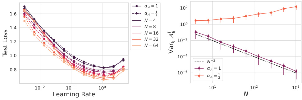
🔼 This figure shows the results of experiments investigating the effect of scaling the dimension per head (N) on hyperparameter transfer and the variance of attention variables across different heads. Panel (a) demonstrates that with µP scaling (αA = 1), optimal learning rates transfer well across different values of N. Panel (b) shows that the variance of attention variables across heads decreases with increasing N under µP scaling, suggesting a collapse towards single-head behavior; however, this variance remains high when αA = 1/2.
read the caption
Figure 2: Increasing dimension-per-head N with heads fixed for αA = {1, 1/2}. (a) Both αA = 1 and αA = 1/2 exhibit similar hyperparameter transfer for vision transformers trained on CIFAR-5M over finite N at H = 16. (b) The variance of attention variables across the different heads of a vision transformer after training for 2500 steps on CIFAR-5M. For αA = 1 the variance of attention variables decays at rate O(N−2) and for αA = 1/2 the variance does not decay with N.

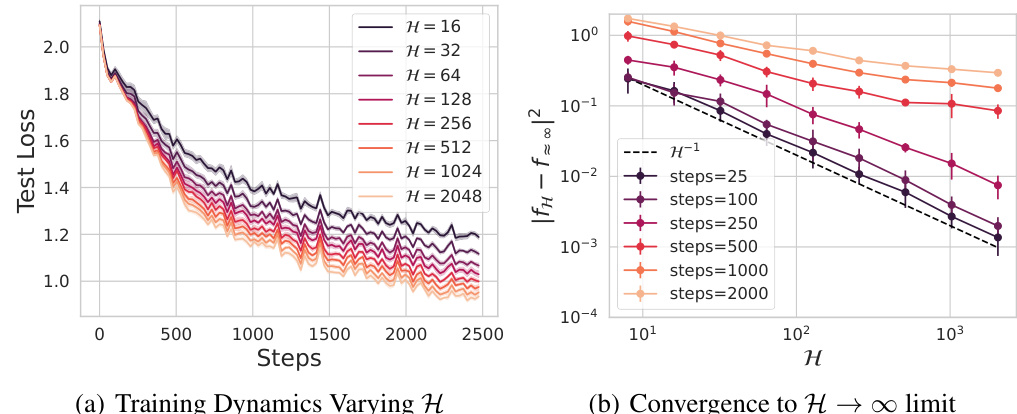
🔼 This figure shows the convergence of the initial kernels and the distribution of attention variables (Ah) as the number of heads (H) approaches infinity. Subfigure (a) demonstrates the convergence of the residual stream kernel Hss′(x, x′) at a rate of O(H−1) in an 8-layer, 4-dimensional vision transformer. Subfigures (b) and (c) illustrate the distribution of Ah for different values of N (dimension per head). Subfigure (b) (N=1) shows a non-Gaussian distribution for small N, while (c) (N=16) shows that as N gets larger, the distribution approaches a Gaussian. The results illustrate the impact of scaling parameters on the initial state of the transformer network.
read the caption
Figure 3: The initial kernels converge as H → ∞ and are determined by (possibly non-Gaussian) distributions of Ah over heads in each layer. (a) Convergence of Hss′(x, x′) = h(x)h(x′) in a L = 8, N = 4 vision transformer at initialization at rate O(H−1). (b) The density of Ah entries over heads at fixed spatial location converges as H → ∞ but is non-Gaussian for small N. (c) As N → ∞ the initial density of A approaches a Gaussian with variance of order O(N1−2αA).
🔼 This figure explores the impact of scaling the dimension per head (N) while keeping the number of heads (H) constant, using two different scaling exponents for the key/query inner product (αA = 1 and αA = 1/2). The left panel (a) demonstrates hyperparameter transfer, showing consistent performance across different values of N for both αA settings. The right panel (b) illustrates the variance of attention variables across heads, revealing a decay for αA = 1 but no decay for αA = 1/2 as N increases, which highlights the impact of the parameterization choice on attention head behavior during training.
read the caption
Figure 2: Increasing dimension-per-head N with heads fixed for αA = {1, 1/2}. (a) Both αA = 1 and αA = 1/2 exhibit similar hyperparameter transfer for vision transformers trained on CIFAR-5M over finite N at H = 16. (b) The variance of attention variables across the different heads of a vision transformer after training for 2500 steps on CIFAR-5M. For αA = 1 the variance of attention variables decays at rate O(N−2) and for αA = 1/2 the variance does not decay with N.
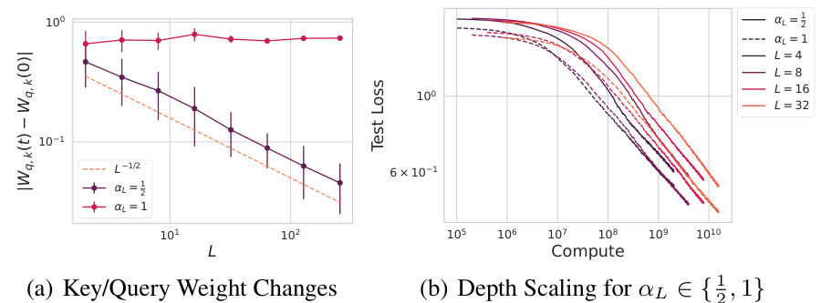
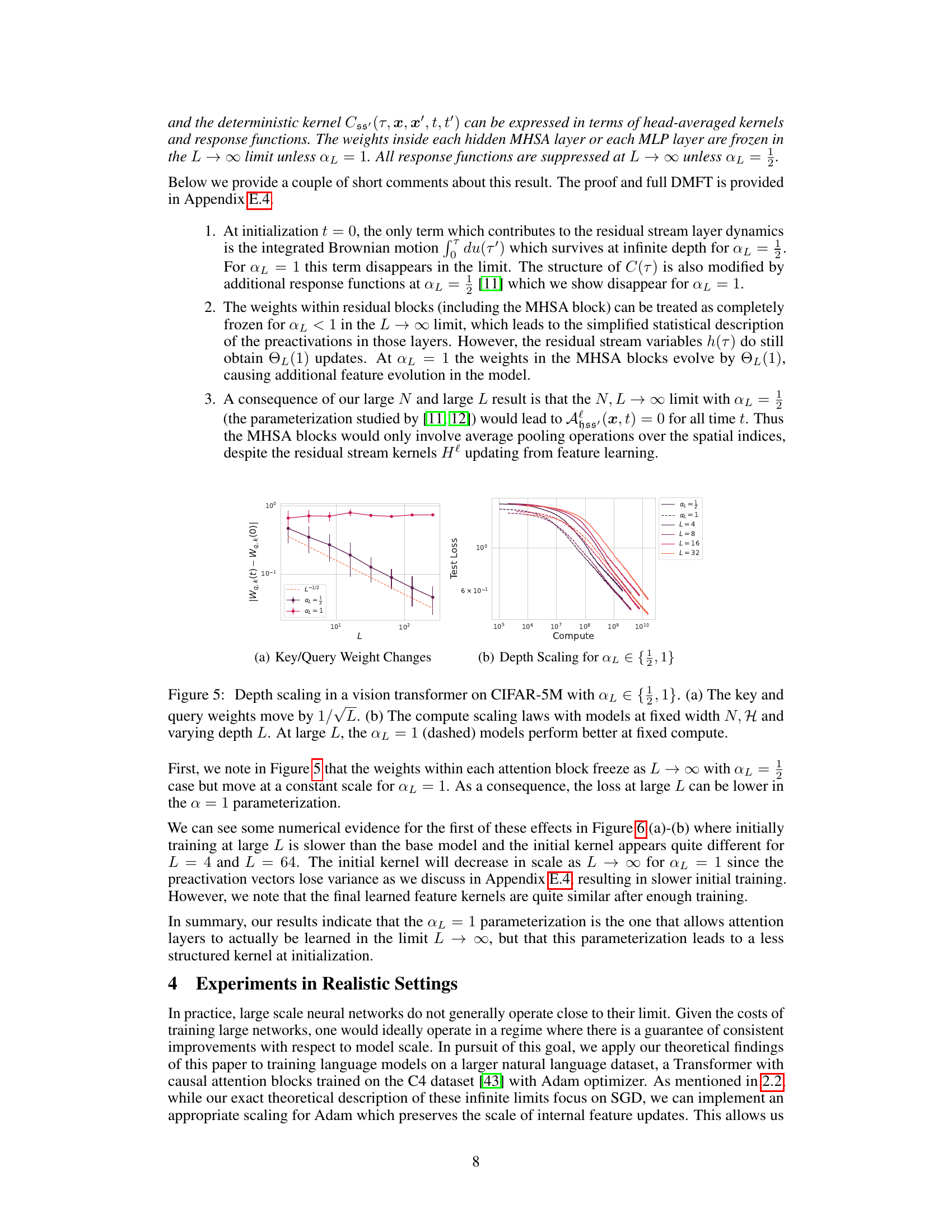
🔼 This figure shows the effects of depth scaling on the performance of a vision transformer model trained on CIFAR-5M dataset. The left panel (a) displays how the key and query weights change with increasing depth L, specifically showing they scale by 1/√L, indicating a scaling law. The right panel (b) shows the compute scaling laws for the models with αL values of 1/2 and 1, demonstrating that models with αL = 1 perform better at a fixed compute budget as depth L increases.
read the caption
Figure 5: Depth scaling in a vision transformer on CIFAR-5M with αL ∈ {1/2,1}. (a) The key and query weights move by 1/√L. (b) The compute scaling laws with models at fixed width N, H and varying depth L. At large L, the αL = 1 (dashed) models perform better at fixed compute.

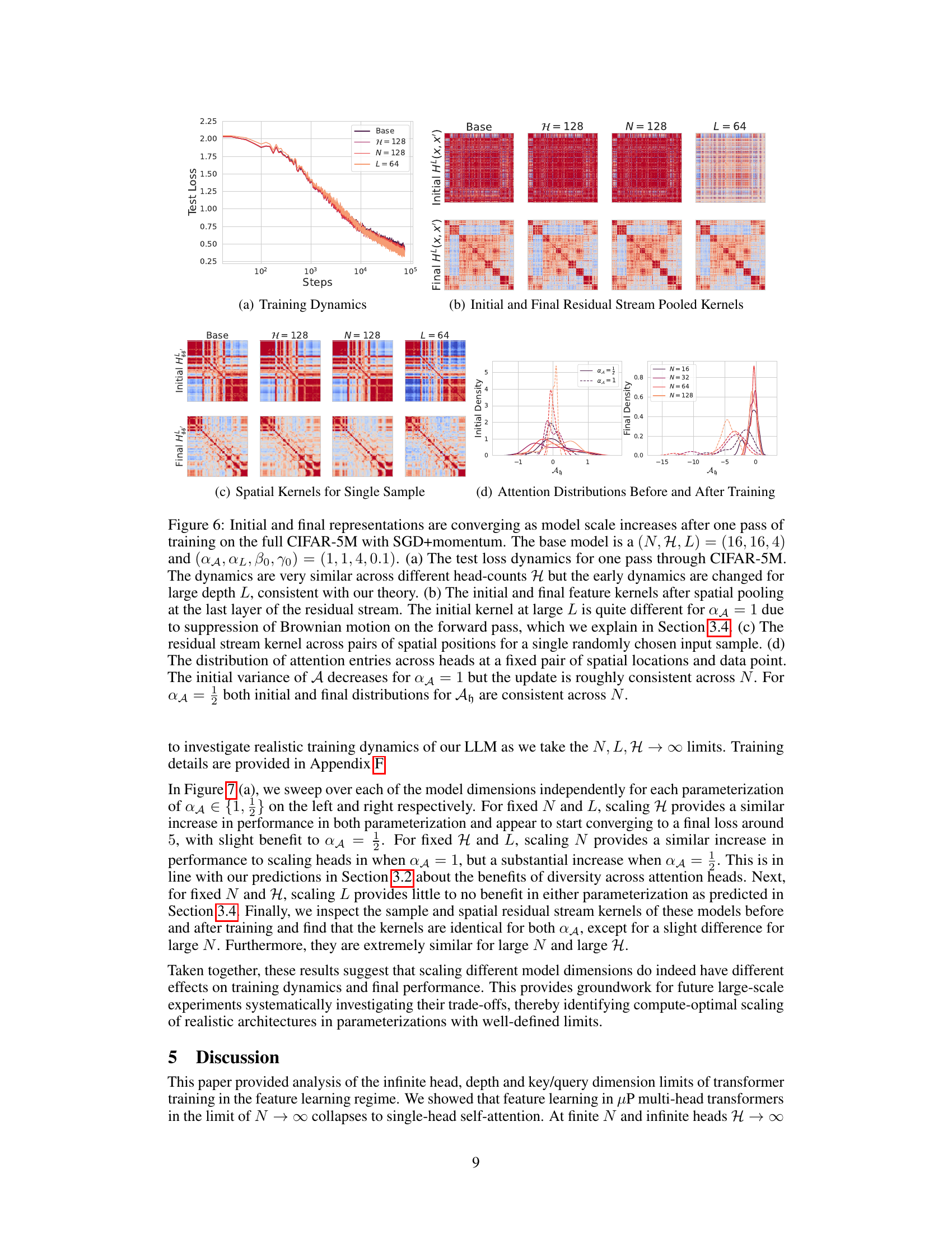
🔼 This figure visualizes the convergence of initial and final representations as the model scales increase after one training pass on the CIFAR-5M dataset. It shows how test loss, residual stream pooled kernels, spatial kernels for a single sample, and attention distributions evolve across various model sizes (N, H, L) and scaling parameters (αA, αL, β0, γ0). The plots demonstrate convergence as model size increases, although the initial kernel at large L exhibits some differences related to Brownian motion suppression under certain parameterizations. The figure corroborates the theoretical analysis presented in the paper, highlighting the impact of different scaling strategies on training dynamics.
read the caption
Figure 6: Initial and final representations are converging as model scale increases after one pass of training on the full CIFAR-5M with SGD+momentum. The base model is a (N, H, L) = (16, 16, 4) and (αA, αL, β0, γ0) = (1, 1, 4, 0.1). (a) The test loss dynamics for one pass through CIFAR-5M. The dynamics are very similar across different head-counts H but the early dynamics are changed for large depth L, consistent with our theory. (b) The initial and final feature kernels after spatial pooling at the last layer of the residual stream. The initial kernel at large L is quite different for αA = 1 due to suppression of Brownian motion on the forward pass, which we explain in Section 3.4. (c) The residual stream kernel across pairs of spatial positions for a single randomly chosen input sample. (d) The distribution of attention entries across heads at a fixed pair of spatial locations and data point. The initial variance of A decreases for αA = 1 but the update is roughly consistent across N. For αA = ½ both initial and final distributions for Ah are consistent across N.
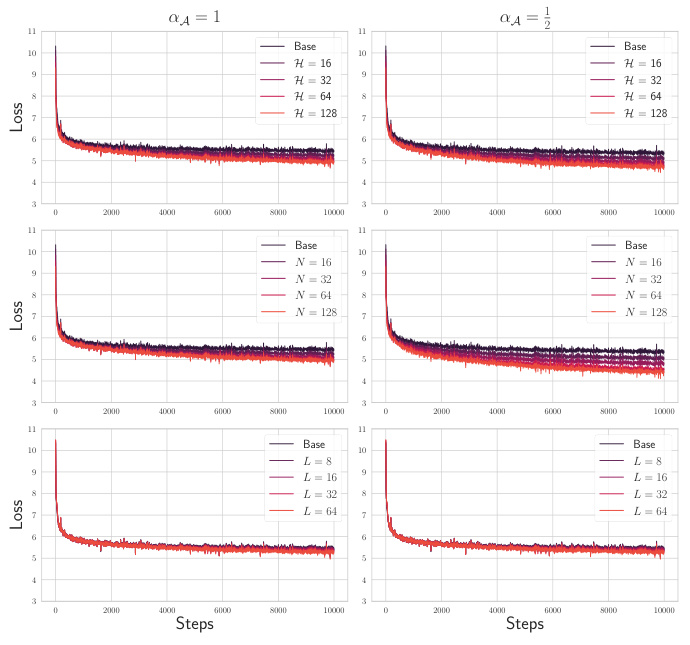
🔼 Figure 7 shows the results of experiments on a causal language model trained on the C4 dataset. It demonstrates how the training dynamics and learned representations change as the model’s size (number of heads, key/query dimension, and depth) increases. The plots highlight differences in performance when scaling model dimensions using different scaling parameters (α = 1 and α = 1/2), revealing the best scaling strategies for optimizing performance at various model sizes.
read the caption
Figure 7: Training dynamics and initial/final representations of decoder only language models trained on C4 converge with increasing model scale. The base model has (N, H, L) = (8,8, 4) and (α₁, β₀, γ₀) = (1, 4, 0.25) and α ∈ {1, ½}. (a) Train loss dynamics after 10000 steps on C4 using Adam optimizer. The dynamics improve consistently when scaling H for both values of α, with slight benefit to α = 1. Scaling N reveals a significant advantage to setting α = ½. Scaling L provides little improvement for either parameterization of α. (b) Initial and final residual stream kernels for the final token across samples for Base, H = 128, N = 128, and L = 64 models. The first row is at initialization. The second and third rows are after training with α ∈ {1, ½} respectively. (c) Initial and final feature kernels across pairs of tokens for a single randomly chosen input sample. Note both types of kernels are identical across α except for a slight difference at large N.

🔼 This figure shows the results of experiments on a decoder-only language model trained on the C4 dataset. It demonstrates the effects of scaling the model’s dimensions (number of heads H, key/query dimension N, and depth L) on training dynamics and learned representations (kernels). Subfigures (a), (b), and (c) show the training loss, the final token kernels across samples and tokens within a sample respectively, for various model sizes. The results suggest that scaling N significantly improves performance, while scaling H leads to modest improvements and scaling L has limited effect. The different αA parameterizations (1 and 1/2) yield similar overall trends but some differences in detail are observed.
read the caption
Figure 7: Training dynamics and initial/final representations of decoder only language models trained on C4 converge with increasing model scale. The base model has (N, H, L) = (8,8, 4) and (αA, β0, γ0) = (1, 4, 0.25) and αA ∈ {1, 1/2}. (a) Train loss dynamics after 10000 steps on C4 using Adam optimizer. The dynamics improve consistently when scaling H for both values of αA, with slight benefit to αA = 1. Scaling N reveals a significant advantage to setting αA = 1/2. Scaling L provides little improvement for either parameterization of αA. (b) Initial and final residual stream kernels for the final token across samples for Base, H = 128, N = 128, and L = 64 models. The first row is at initialization. The second and third rows are after training with αA ∈ {1, 1/2} respectively. (c) Initial and final feature kernels across pairs of tokens for a single randomly chosen input sample. Note both types of kernels are identical across αA except for a slight difference at large N.

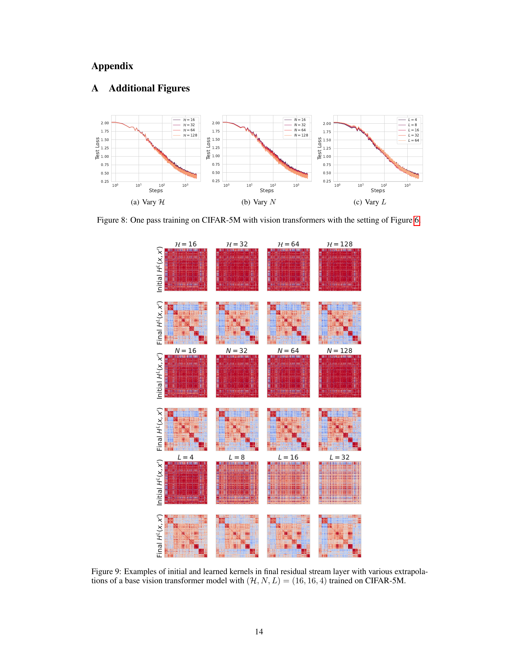
🔼 This figure shows the training curves for vision transformers trained on the CIFAR-5M dataset. It demonstrates how the test loss changes over training steps when varying the number of heads (H), the number of dimensions per head (N), and the depth (L) of the transformer model. Each subplot shows the training curves under different parameterizations of these three hyperparameters, highlighting the relationship between model scale and training dynamics.
read the caption
Figure 8: One pass training on CIFAR-5M with vision transformers with the setting of Figure 6.
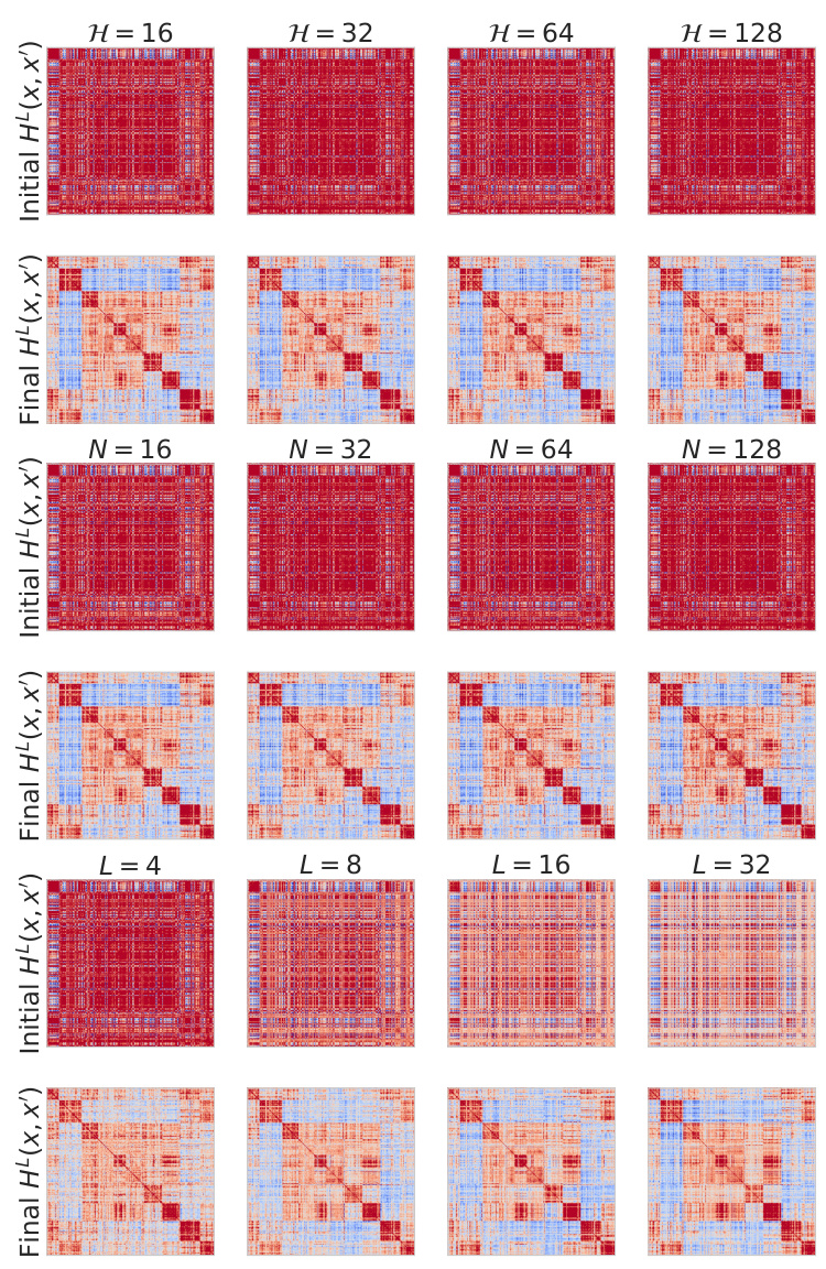
🔼 This figure visualizes the spatial kernels before and after training of a vision transformer model. The kernels are shown for various values of H (number of heads), N (dimension per head), and L (depth). The heatmap shows kernel values across different spatial locations, revealing how these change during training and how model parameters affect them. Specifically, it illustrates the effect of different hyperparameter scalings on the learned representations.
read the caption
Figure 10: Spatial kernels for a single test point before and after training across H, N, L values.

🔼 This figure visualizes spatial kernels before and after training a vision transformer on the CIFAR-5M dataset. It shows how these kernels change across different model sizes by varying the number of heads (H), the dimension per head (N), and the depth (L) of the network. Each subplot presents a heatmap representing the kernel, where the color intensity represents the kernel value. The top row shows the initial kernels, and the bottom row shows the kernels after training. The pattern changes suggest how the model’s representation of spatial relationships evolves during training and how this evolution depends on the architectural choices for H, N and L.
read the caption
Figure 10: Spatial kernels for a single test point before and after training across H, N, L values.

🔼 This figure shows the results of experiments investigating the impact of increasing the dimension per head (N) on vision transformer training. Subfigure (a) demonstrates hyperparameter transfer, showing that models with different values of N maintain similar performance when scaled appropriately (αA = 1, 1/2). Subfigure (b) examines the variance of attention across different heads. With αA = 1, the variance decreases as N increases, suggesting that the network effectively collapses to a single-head attention mechanism in the large N limit. However, with αA = 1/2, this variance does not decrease, indicating head diversity is maintained.
read the caption
Figure 2: Increasing dimension-per-head N with heads fixed for αA = {1, 1/2}. (a) Both αA = 1 and αA = 1/2 exhibit similar hyperparameter transfer for vision transformers trained on CIFAR-5M over finite N at H = 16. (b) The variance of attention variables across the different heads of a vision transformer after training for 2500 steps on CIFAR-5M. For αA = 1 the variance of attention variables decays at rate O(N−2) and for αA = 1/2 the variance does not decay with N.
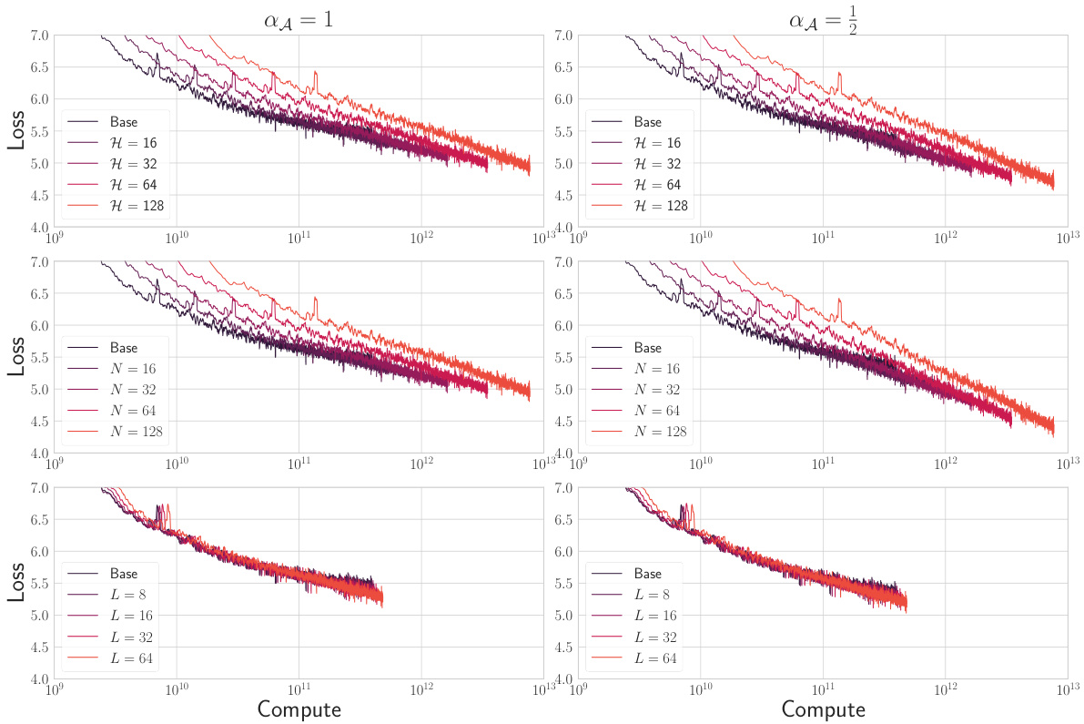
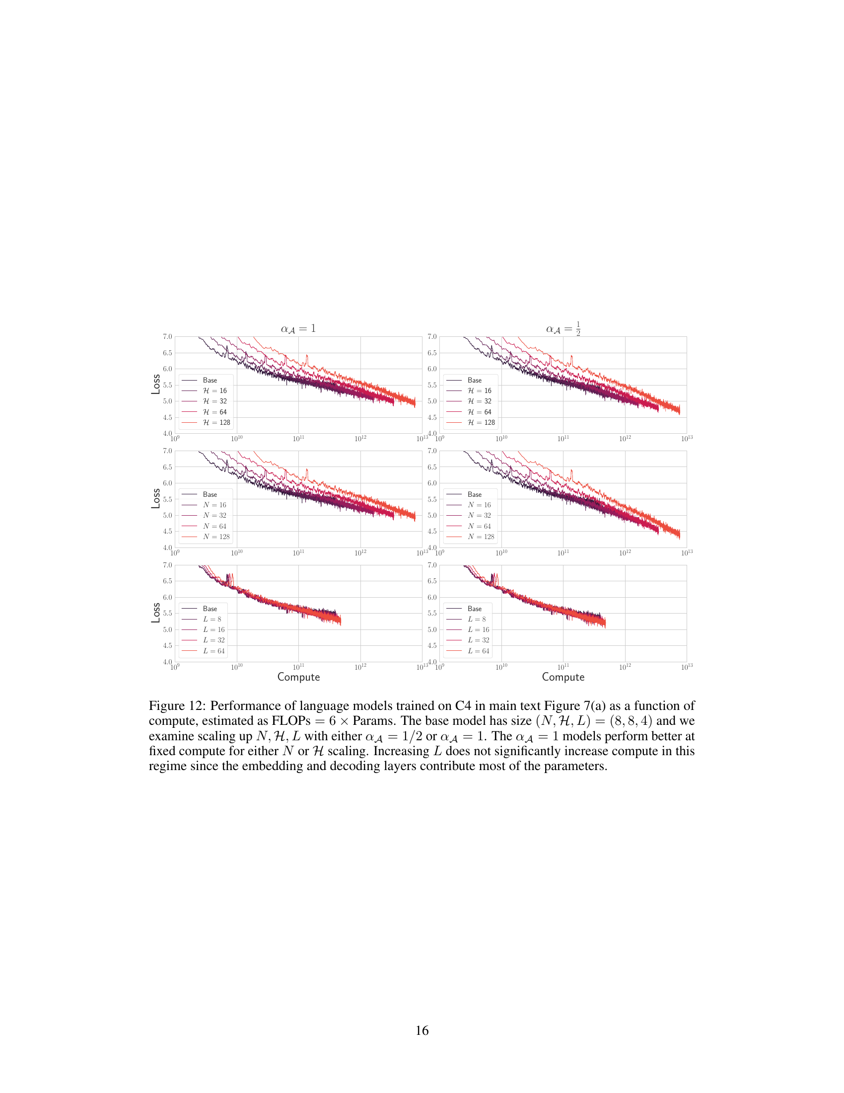
🔼 The figure shows the performance of language models trained on the C4 dataset, in terms of loss, as a function of compute (estimated as FLOPs = 6 * number of parameters). Different model sizes were tested, varying the key/query dimension (N), number of heads (H), and depth (L), while using two different scaling exponents (αA = 1/2 and αA = 1). The results indicate that using αA = 1 leads to better performance at a fixed compute, particularly when scaling N or H. Scaling L did not significantly increase compute due to the dominant contribution of embedding and decoding layers to the total number of parameters.
read the caption
Figure 12: Performance of language models trained on C4 in main text Figure 7(a) as a function of compute, estimated as FLOPs = 6 × Params. The base model has size (N, H, L) = (8,8, 4) and we examine scaling up N, H, L with either αA = 1/2 or αA = 1. The αA = 1 models perform better at fixed compute for either N or H scaling. Increasing L does not significantly increase compute in this regime since the embedding and decoding layers contribute most of the parameters.
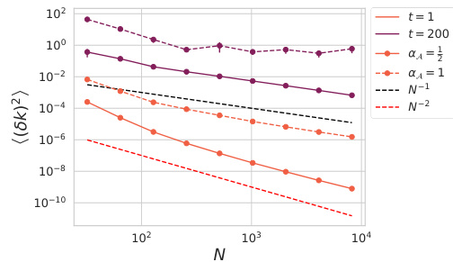
🔼 This figure shows the results of experiments investigating the effect of increasing the dimension per head (N) on hyperparameter transfer and attention variance in vision transformers. Panel (a) demonstrates that with either key/query scaling exponent (aλ), similar hyperparameters work across different values of N, exhibiting hyperparameter transfer. Panel (b) shows that only with the mean field scaling exponent (aλ = 1) does the variance of attention variables across heads decay with increasing N, while it remains constant for aλ = 1/2.
read the caption
Figure 2: Increasing dimension-per-head N with heads fixed for aλ = {1, 1/2}. (a) Both aλ = 1 and aλ = 1/2 exhibit similar hyperparameter transfer for vision transformers trained on CIFAR-5M over finite N at H = 16. (b) The variance of attention variables across the different heads of a vision transformer after training for 2500 steps on CIFAR-5M. For aλ = 1 the variance of attention variables decays at rate O(N−2) and for aλ = 1/2 the variance does not decay with N.
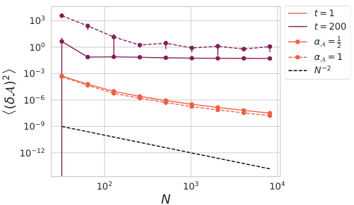
🔼 This figure shows the results of experiments investigating the effect of increasing the dimension per head (N) on hyperparameter transfer and attention variance in vision transformers. Subfigure (a) demonstrates that with either scaling of the key-query inner product (αA = 1 or αA = 1/2), similar hyperparameter transfer occurs across different values of N. Subfigure (b) shows that when αA = 1, attention variance decays with increasing N, suggesting that the heads of the network converge towards similar behaviour; however, when αA = 1/2, attention variance does not decrease, indicating that heads maintain diversity.
read the caption
Figure 2: Increasing dimension-per-head N with heads fixed for αA = {1, 1/2}. (a) Both αA = 1 and αA = 1/2 exhibit similar hyperparameter transfer for vision transformers trained on CIFAR-5M over finite N at H = 16. (b) The variance of attention variables across the different heads of a vision transformer after training for 2500 steps on CIFAR-5M. For αA = 1 the variance of attention variables decays at rate O(N−2) and for αA = 1/2 the variance does not decay with N.
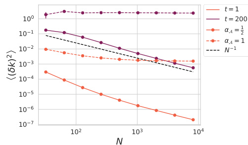
🔼 This figure shows the impact of increasing the dimension per head (N) on hyperparameter transfer and attention variance across heads. Panel (a) demonstrates that using the µP scaling (aA = 1) leads to similar performance across varying N, while Panel (b) shows that the attention variance decays with N only when aA = 1, implying that identical dynamics only occurs when µP scaling is used.
read the caption
Figure 2: Increasing dimension-per-head N with heads fixed for aA = {1,}. (a) Both aA = 1 and aA = exhibit similar hyperparameter transfer for vision transformers trained on CIFAR-5M over finite N at H = 16. (b) The variance of attention variables across the different heads of a vision transformer after training for 2500 steps on CIFAR-5M. For aA = 1 the variance of attention variables decays at rate O(N−2) and for aA = the variance does not decay with N.

🔼 This figure demonstrates the impact of scaling the dimension per head (N) on hyperparameter transfer and attention variance across heads in vision transformers. Panel (a) shows that with the µP scaling (α₄ = 1), similar performance is achieved across different values of N, indicating hyperparameter transfer. In contrast, with α₄ = 1/2, this transferability is lost. Panel (b) visualizes the variance of attention variables across different heads, showing that it decays rapidly with increasing N for α₄ = 1 but remains relatively constant for α₄ = 1/2.
read the caption
Figure 2: Increasing dimension-per-head N with heads fixed for α₄ = {1, 3}. (a) Both α₄ = 1 and α₄ = 1/2 exhibit similar hyperparameter transfer for vision transformers trained on CIFAR-5M over finite N at H = 16. (b) The variance of attention variables across the different heads of a vision transformer after training for 2500 steps on CIFAR-5M. For α₄ = 1 the variance of attention variables decays at rate O(N⁻²) and for α₄ = 1/2 the variance does not decay with N.

🔼 This figure shows the results of experiments investigating the effect of scaling the dimension per head (N) on hyperparameter transfer and attention variance across multiple heads in vision transformers. Part (a) demonstrates that with the appropriate scaling (αA=1 and αA=1/2), similar hyperparameter performance is observed across different values of N. Part (b) shows that for αA=1 (μP scaling), the variance of attention across heads decreases quadratically with increasing N while for αA=1/2 this is not the case.
read the caption
Figure 2: Increasing dimension-per-head N with heads fixed for αA = {1, 3}. (a) Both αA = 1 and αA = 1/2 exhibit similar hyperparameter transfer for vision transformers trained on CIFAR-5M over finite N at H = 16. (b) The variance of attention variables across the different heads of a vision transformer after training for 2500 steps on CIFAR-5M. For αA = 1 the variance of attention variables decays at rate O(N−2) and for αA = 1/2 the variance does not decay with N.
More on tables

🔼 This table presents the learning rate scaling for SGD and Adam optimizers to maintain consistent feature updates across different model sizes (N, H, L). It also shows the necessary rescaling of the first layer’s weights and multipliers, dependent on the optimizer and parameterization.
read the caption
Table 1: The learning rates which should be applied to obtain the correct scale of updates for SGD or Adam optimizers. In addition, the weight variance and multiplier for the first layer may need to be rescaled (relative to eq (5)) with width/depth depending on the parameterization and optimizer.

🔼 This table shows two different ways to scale the attention layer exponent (αA) to achieve approximately constant updates to the attention matrices (Ah) during training. The first uses the mean-field parameterization (μP) with αA = 1. This method, while resulting in non-negligible updates, causes all attention heads to behave identically and results in zero attention matrices (Ah) at initialization. The second approach uses αA = ½, which produces random, but non-negligible attention matrix updates.
read the caption
Table 3: Two interesting choices of scaling for the attention layer exponent αA which give approximately constant updates to the attention matrices Ah. The μP scaling αA = 1 causes the entries of the key/query vector entries to move non-negligibly but causes all heads to be identical (and all A = 0) at initialization. Scaling instead with αA = ½ causes the A variables to be random but still non-negligibly updated under training.
Full paper#
