Linear Transformers are Versatile In-Context Learners

↗ OpenReview ↗ NeurIPS Homepage ↗ Hugging Face ↗ Chat

TL;DR

#

Key Takeaways

#

Why does it matter?

#

This paper is crucial because it reveals the surprising ability of linear transformers to discover sophisticated optimization algorithms implicitly. This challenges our understanding of transformer functionality and opens new avenues for algorithm design and optimization in machine learning.

Visual Insights

#

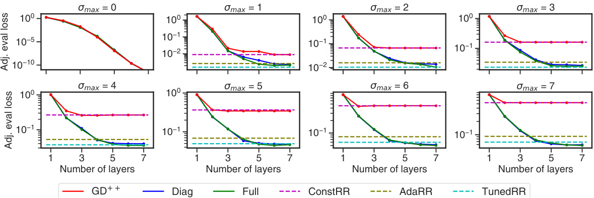
The figure displays the performance of various models on a noisy linear regression task. Each model is evaluated across a range of maximum noise levels (σmax) and different numbers of layers. The plot shows that linear transformers (both full and diagonal attention variants) significantly outperform models designed for fixed noise levels and even a tuned ridge regression model. The diagonal attention and full attention models achieve comparable results, while the fixed-noise model (GD++) performs poorly.

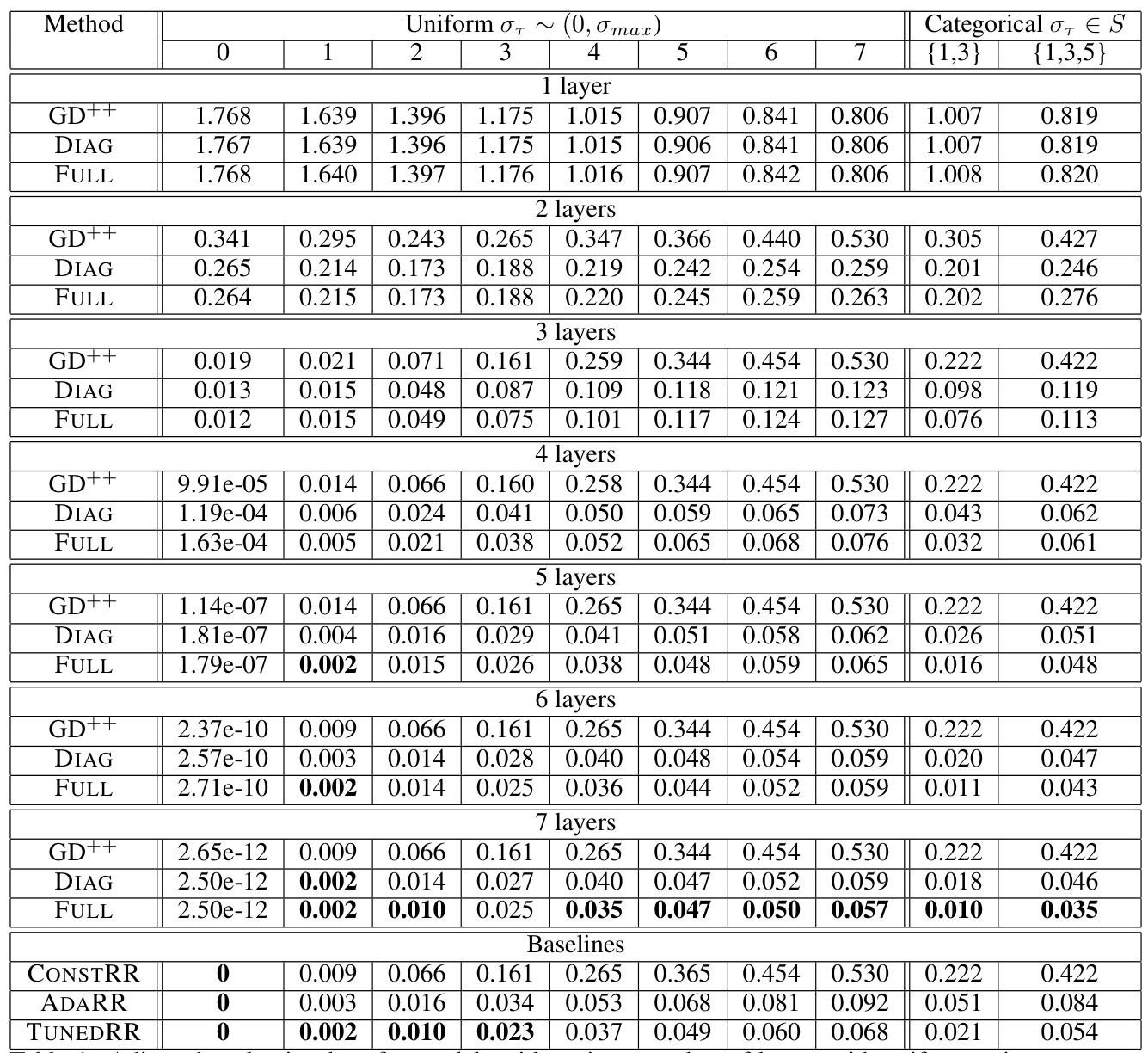
This table presents a comprehensive comparison of the adjusted evaluation loss achieved by different linear transformer models (GD++, DIAG, FULL) across various configurations. The configurations are defined by the number of layers in the model and the noise variance in the data. For each setup, the lowest adjusted evaluation loss is highlighted in bold. The table also provides a comparison against several baselines (CONSTRR, ADARR, TUNEDRR).

In-depth insights

#

Linear Transformer ICL

#

Research on “Linear Transformer ICL” (In-Context Learning) reveals surprising optimization capabilities within these seemingly simple models. Each layer implicitly performs a form of preconditioned gradient descent, effectively learning a linear regression model. However, the true power lies in their ability to discover sophisticated optimization strategies when faced with noisy data, surpassing many established baselines. Adaptive rescaling and momentum-like behavior emerge from the model’s weights, demonstrating a novel approach to handling varying noise levels. This unexpected adaptability highlights the potential of linear transformers as efficient, effective in-context learners, and suggests exciting avenues for algorithmic discovery and optimization within more complex transformer architectures. The research also reveals a remarkable versatility in solving linear regression problems, indicating that linear transformers could potentially be adapted and improved for more challenging tasks, particularly those involving noisy and uncertain data.

Implicit Optimization

#

The concept of implicit optimization in the context of the provided research paper centers on the observation that transformer networks, particularly linear transformers, appear to implicitly perform optimization algorithms during their forward pass. This is surprising because the networks aren’t explicitly designed to do so; rather, this behavior emerges from the architecture and training process. The paper explores this phenomenon by demonstrating that each layer of a linear transformer implicitly maintains a weight vector for a linear regression problem and can be viewed as performing a sophisticated variant of preconditioned gradient descent. The intriguing aspect is the ability of these models to discover complex and highly effective optimization strategies, especially when dealing with noisy data. This suggests a potential for transformers to uncover novel optimization algorithms that may surpass traditional methods. The research goes further by analyzing how these implicit algorithms incorporate momentum and adaptive rescaling mechanisms based on noise levels. The implications are significant, highlighting the potential for AI to discover and utilize complex optimization strategies without explicit programming, advancing our understanding of both transformers and optimization techniques more broadly.

Noisy Regression

#

The concept of ‘Noisy Regression’ is crucial in evaluating the robustness and generalizability of machine learning models. It acknowledges that real-world data is rarely clean and often contains errors or noise. Successfully handling noisy data is critical for building reliable and accurate models that perform well in unpredictable environments. The paper likely explores different types of noise (e.g., Gaussian, uniform, or categorical) and their impact on the performance of linear transformers as in-context learners. The analysis might investigate how well the implicit optimization algorithms discovered within the linear transformers adapt to various noise levels. This would shed light on the inherent ability of these models to handle uncertainty and potentially reveal novel optimization strategies. A key aspect would be comparing the performance of linear transformers against traditional regression methods (like ridge regression) under noisy conditions, demonstrating their strengths and limitations in noisy settings. The findings would contribute significantly to a deeper understanding of in-context learning, its robustness, and potential for discovering sophisticated optimization techniques.

Adaptive Rescaling

#

The concept of “Adaptive Rescaling” within the context of the research paper, likely refers to a mechanism where the model dynamically adjusts its internal parameters based on the level of noise present in the input data. This is crucial for handling noisy data, a common challenge in machine learning. The adaptive nature implies the model isn’t using a fixed scaling factor, but rather learns to modify the scaling based on observations from the input. This is a significant advancement because it avoids the limitations of fixed-scaling methods, which struggle to perform well across various noise levels. The implementation likely involves analyzing the data’s noise characteristics and then using this information to adjust internal weights or activation functions. Such an adaptive approach mimics sophisticated optimization strategies found in more complex algorithms, showing the surprising capabilities even simple linear transformers possess. The core insight here is that even a seemingly straightforward architecture can exhibit complex behavior when trained on challenging problems, suggesting that further research could uncover many more powerful, implicit algorithms within neural networks. The adaptive rescaling mechanism is key to the model’s ability to effectively handle noise variance, a finding that significantly contributes to a broader understanding of in-context learning and implicit algorithm discovery.

Diagonal Attention

#

Employing diagonal attention mechanisms in transformer models presents a compelling trade-off between computational efficiency and performance. Restricting attention weights to a diagonal matrix significantly reduces the number of parameters, leading to faster training and inference times. This simplification is particularly beneficial for resource-constrained environments or when deploying models on edge devices. While this approach might seem overly simplistic, it offers surprising performance. The paper shows that even with this constraint, linear transformers can still effectively solve complex regression problems, often matching or exceeding the performance of models with full attention matrices in certain scenarios, especially in noisy data settings. The reduced parameter space also makes the diagonal attention model easier to interpret, which is particularly helpful for understanding the internal mechanisms employed by transformers for in-context learning. However, it is crucial to acknowledge the limitation of reduced expressiveness due to the constraint. This might lead to suboptimal solutions or lower performance in tasks demanding greater expressivity and subtle relationships in data. Further research could explore the theoretical limitations and potential enhancements to diagonal attention to broaden its applicability and effectiveness across a broader range of tasks.

More visual insights

#

More on figures

This figure compares the performance of different models (GD++, Diag, Full, ConstRR, AdaRR, TunedRR) on a noisy linear regression task. It shows how the adjusted evaluation loss varies with the number of layers in the model and different maximum noise levels (σmax). The key takeaway is that linear transformers (Diag and Full) significantly outperform simpler baselines, especially with higher noise levels and a greater number of layers.

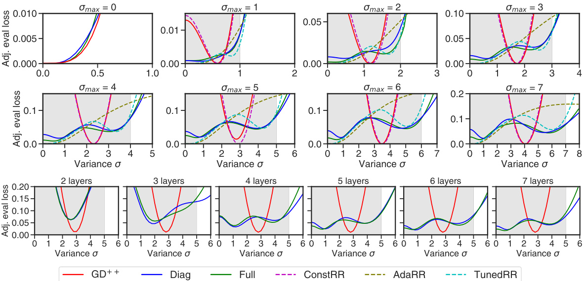
This figure displays the in-context learning performance of various models on noisy linear regression problems with different numbers of layers and noise variance distributions. The top section shows the overall loss for models with different layer counts and a per-variance profile for 7-layer models. The bottom section presents per-variance profiles for models with varying layer counts (2-7 layers). The shaded gray regions indicate in-distribution noise variance. The plot helps to analyze how the model performance changes as the number of layers and the noise variance change.

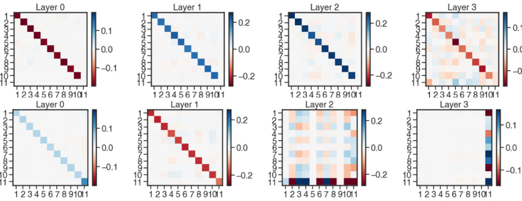
This figure shows the weight matrices (Q and P) for a 4-layer linear transformer with full parametrization. The model was trained using categorical noise with values of 1 and 3. The top half displays the Q matrix across layers 0-3, while the bottom half displays the P matrix across the same layers. Each subplot represents a layer, showing the weight matrix’s values as a heatmap. The color scale represents the magnitude of the weights, with darker colors indicating larger magnitudes. The visualization helps understand how the weights evolve across layers during the learning process within the linear transformer model for this specific noise distribution.

The figure displays the adjusted evaluation loss for linear transformer models (GD++, Diag, Full) with varying numbers of layers (1 to 7) trained on data with mixed noise variance. The x-axis represents the number of layers, and the y-axis shows the adjusted evaluation loss. Each line represents a different number of layers, and the shaded area around each line shows the variance over 5 training seeds. The figure demonstrates that, for all model types, the loss consistently decreases as the number of layers increases, indicating that the models learn effectively from the noisy data, with a more consistent and accurate decrease in error as the number of layers increases.

This figure shows the unadjusted evaluation loss for different models as a function of the noise variance. The unadjusted loss is calculated directly from the loss function, without any adjustments for the oracle loss (the best possible solution given the noise variance). It is difficult to compare the methods using this loss because the scale of the loss is heavily influenced by the amount of noise.

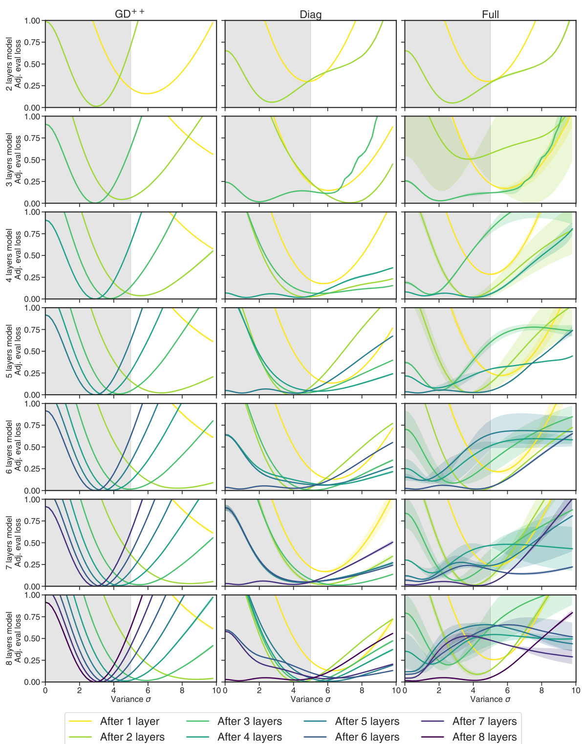
This figure shows the performance of three different linear transformer models (GD++, Diag, and Full) across various noise levels (variance σ) and different numbers of layers. The x-axis represents the variance of the noise, and the y-axis represents the adjusted evaluation loss. Each line represents the model’s performance after a specific number of layers, allowing a visualization of how model performance changes as layers are added and as noise levels vary. The shaded regions represent the standard deviation. It reveals how the models’ ability to handle noise changes with increasing depth and reveals different behaviors and convergence patterns for each model type.

Full paper

#