TL;DR#
Many machine learning models assume that training and test data come from the same distribution. However, this is often not true in real-world scenarios, especially when dealing with time-series data, where the data distribution can change over time. This is called a ’temporal distribution shift,’ and it leads to a significant drop in the performance of the model. Until now, there hasn’t been a reliable method that performs consistently well in tabular datasets with temporal distribution shifts.
This paper introduces a new approach called ‘Drift-Resilient TabPFN’ to tackle this problem. This method cleverly uses ‘in-context learning’ where the entire training dataset is fed as input to a neural network, which then predicts the outcome directly. The network is trained on many synthetic datasets generated from a model that simulates how the data distribution changes over time. The results show that Drift-Resilient TabPFN significantly outperforms existing methods across multiple real-world datasets, demonstrating significant improvements in terms of accuracy and other evaluation metrics.
Key Takeaways#
Why does it matter?#
This paper is crucial for researchers dealing with temporal distribution shifts in tabular data, a common real-world problem largely unsolved by existing methods. It introduces a novel and efficient approach, paving the way for improved out-of-distribution predictions in various applications, from healthcare to finance. The in-context learning framework presented offers a fresh perspective and encourages further exploration of ICL techniques in this domain.
Visual Insights#
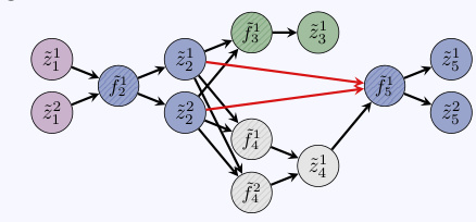
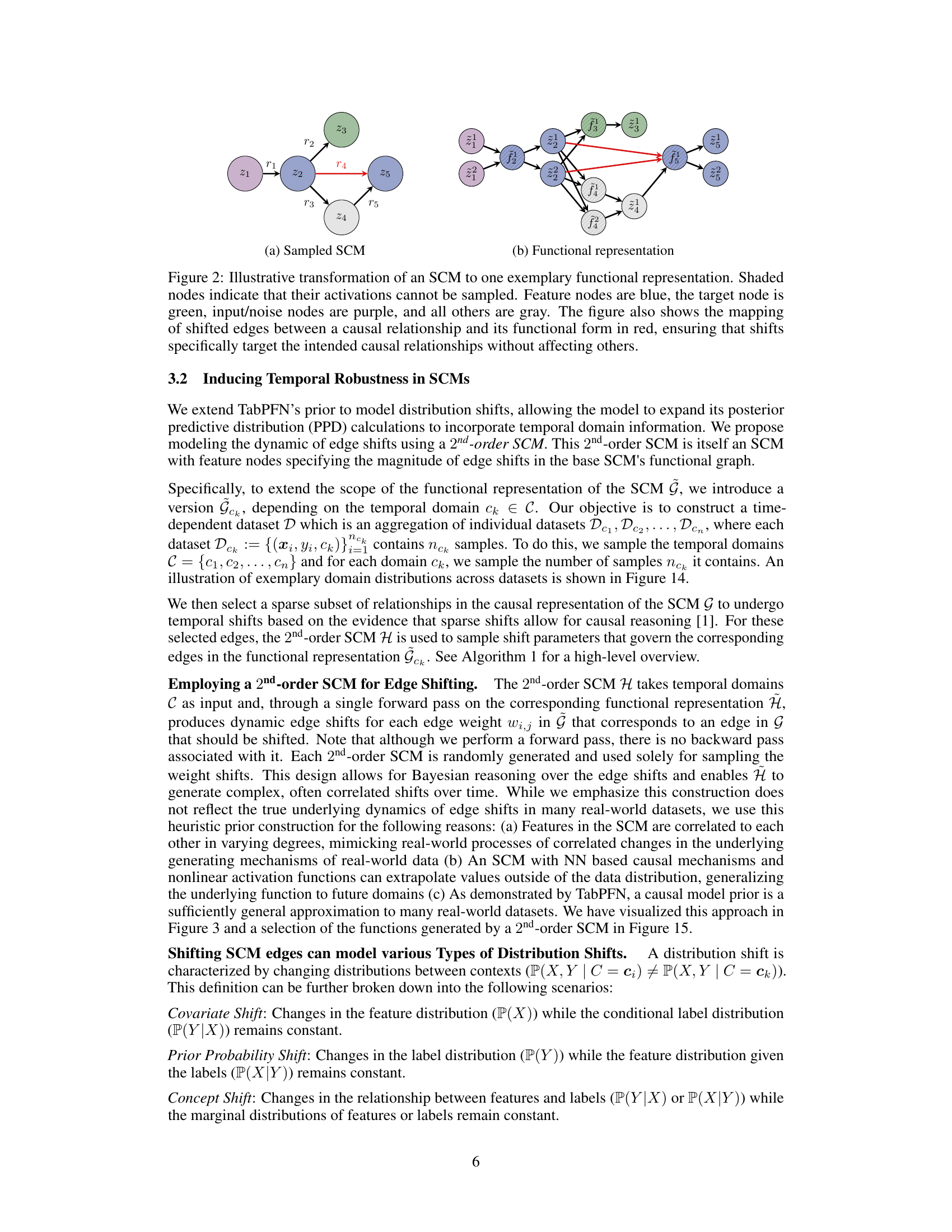
🔼 This figure illustrates the transformation from a structural causal model (SCM) graph representation to its equivalent functional representation. It highlights how the SCM’s nodes (mechanisms) and edges (relationships) translate into a functional graph where each node represents a scalar value and edges represent linear connections. The figure also showcases how edge shifts, represented in red, are specifically applied to target causal relationships within the functional graph.
read the caption
Figure 2: Illustrative transformation of an SCM to one exemplary functional representation. Shaded nodes indicate that their activations cannot be sampled. Feature nodes are blue, the target node is green, input/noise nodes are purple, and all others are gray. The figure also shows the mapping of shifted edges between a causal relationship and its functional form in red, ensuring that shifts specifically target the intended causal relationships without affecting others.

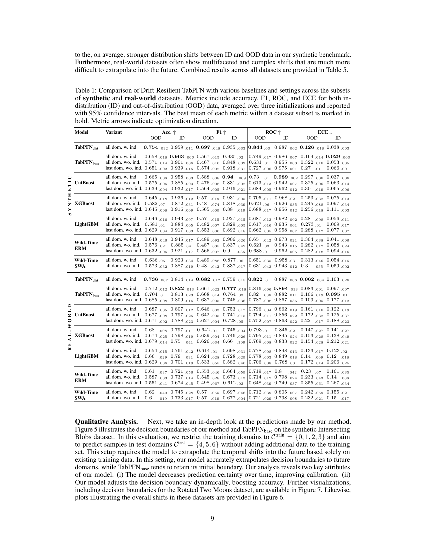
🔼 This table presents a quantitative comparison of the proposed Drift-Resilient TabPFN model against several baseline methods across a range of synthetic and real-world datasets. For each dataset subset (synthetic and real-world), the table shows the performance of each model using metrics such as accuracy, F1-score, ROC AUC, and Expected Calibration Error (ECE), both for in-distribution (ID) and out-of-distribution (OOD) data. The best-performing model for each metric within each dataset subset is highlighted in bold. The results are averaged over three runs with 95% confidence intervals to reflect the statistical significance.
read the caption
Table 1: Comparison of Drift-Resilient TabPFN with various baselines and settings across the subsets of synthetic and real-world datasets. Metrics include accuracy, F1, ROC, and ECE for both in-distribution (ID) and out-of-distribution (OOD) data, averaged over three initializations and reported with 95% confidence intervals. The best mean of each metric within a dataset subset is marked in bold. Metric arrows indicate optimization direction.
In-depth insights#
Tabular Drift Handling#
Tabular data, ubiquitous in real-world applications, presents unique challenges for drift handling due to its inherent structure and the complexities of feature interactions. Existing methods often struggle to effectively model and extrapolate distribution shifts in tabular data, leading to performance degradation in real-world scenarios. A key issue is that traditional approaches frequently rely on neural networks, which, while powerful, haven’t consistently surpassed tree-based methods in tabular data. Innovative approaches that leverage in-context learning (ICL) and incorporate prior knowledge about data generating mechanisms (e.g., using Structural Causal Models) hold significant promise for addressing these challenges. Such methods can learn the learning algorithm itself, adapting more effectively to unseen temporal shifts and requiring less data for training. A critical aspect is handling various types of distribution shifts (covariate, prior probability, concept) within the tabular context. Furthermore, scalable methods are crucial, particularly when dealing with large datasets common in real-world applications. Research in this area needs to focus on developing methods that are both robust and efficient, while maintaining explainability and ease of use.
In-Context Learning#
In-context learning (ICL), a core concept in this research, is explored through the lens of prior-data fitted networks (PFNs). The approach leverages millions of synthetic datasets, generated from a structural causal model (SCM) prior, to train a transformer model. Instead of learning a specific predictive function, the model learns a generalized learning algorithm that can adapt to unseen data. This is accomplished by training the model on complete datasets, rather than individual samples, enabling it to directly learn the underlying relationships between features and labels and how these relationships might shift. Temporal distribution shifts are modeled by introducing a secondary SCM that gradually modifies the parameters of the primary SCM over time. This approach allows the model to not only adapt to but also extrapolate temporal changes which is a significant advantage over traditional methods that solely consider static data distributions. The effectiveness of ICL in handling tabular data exhibiting temporal shifts is a novel contribution highlighted by the study. The results demonstrate the method’s robustness and ability to learn robust algorithms for addressing out-of-distribution prediction challenges.
Causal Model Priors#
The concept of “Causal Model Priors” in machine learning is crucial for addressing the limitations of traditional methods that assume independent and identically distributed data. By incorporating causal knowledge into the model, we move beyond simple correlation and towards understanding the underlying mechanisms generating the data. This allows for more robust predictions, especially when dealing with complex real-world scenarios involving temporal shifts in data distribution. Structural Causal Models (SCMs) are a powerful tool for representing these causal relationships, enabling the model to learn how variables interact and how these interactions might change over time. Using SCMs as priors allows for the generation of synthetic datasets that reflect the model’s inductive bias, resulting in improved generalization and out-of-distribution performance. However, carefully choosing the structure and parameters of the SCM prior is essential. An overly simplistic model might fail to capture the subtleties of real-world causal mechanisms, while an overly complex model can be computationally expensive and prone to overfitting. The balance between model expressiveness and computational feasibility is a critical consideration when designing causal model priors for machine learning.
Temporal Extrapolation#
Temporal extrapolation, in the context of this research paper, refers to a model’s ability to predict future trends based on patterns observed in past data. The paper emphasizes that this capability is particularly challenging when dealing with temporal distribution shifts, where the underlying data generating process changes over time. The proposed method, Drift-Resilient TabPFN, aims to address this challenge by using structural causal models (SCM). The SCM framework allows modeling of the underlying data generating process and its evolution, and it uses synthetic data to learn this behavior. Therefore, the ability to extrapolate temporal trends hinges on accurately modeling causal mechanisms and changes to these mechanisms, which in turn enables predictions for unseen future data. This approach appears more effective than the typical methods for temporal domain generalization.
Scalability Challenges#
Scalability is a critical concern in machine learning, particularly when dealing with large datasets or complex models. In the context of temporal distribution shifts, scalability challenges become even more pronounced. The computational cost of training models that can adapt to evolving data distributions can be substantial, especially for methods that require extensive pre-training on synthetic datasets, as is the case with in-context learning approaches. Additionally, the need to continuously update models as new data becomes available adds to the computational burden. The memory footprint of these large models is also a significant concern, especially when limited computing resources are available. Furthermore, the time complexity of inference can be prohibitive for real-time or near real-time applications, particularly when dealing with high-dimensional data. Addressing these scalability issues necessitates careful consideration of model architecture, training strategies, and algorithmic optimizations. Efficient model compression techniques, distributed computing frameworks, and incremental learning algorithms are essential for creating scalable solutions that can handle the complexities of temporal distribution shifts.
More visual insights#
More on figures

🔼 This figure illustrates how the authors’ method incorporates a second-order structural causal model (SCM) to dynamically adjust edge weights in a primary SCM, thereby simulating temporal distribution shifts in data. The 2nd-order SCM takes a temporal domain indicator as input and outputs weight adjustments for edges in the primary SCM. This allows the model to adapt to changes in the underlying causal relationships over time.
read the caption
Figure 3: Diagram illustrating the integration of a 2nd-order SCM for adaptive edge shifting across evolving temporal domains. On the right, the primary network G generates data samples over multiple time domains, with red arrows indicating shifted edges. On the left, the 2nd-order SCM - an auxiliary network Ĥ - takes an input domain ck ∈ C and outputs parameters to adaptively shift each edge weight wi in the base network.

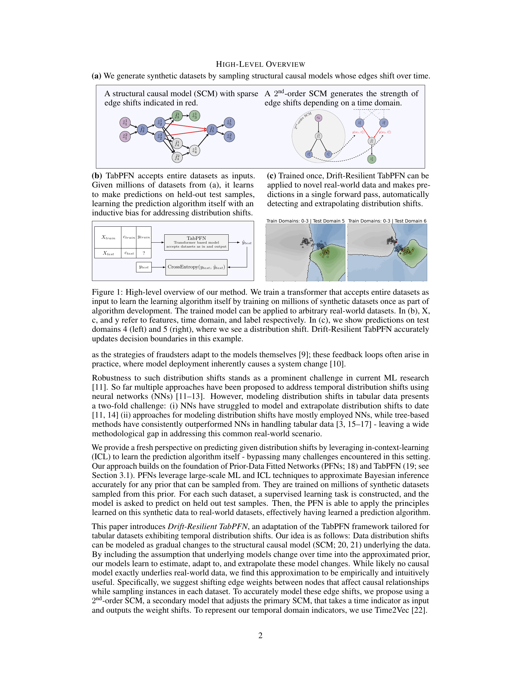
🔼 This figure provides a high-level overview of the proposed Drift-Resilient TabPFN method. It shows how a transformer model is trained on synthetic datasets to learn a prediction algorithm that is robust to distribution shifts. The model accepts the entire dataset as input and makes predictions in a single forward pass. The figure illustrates the method’s ability to adapt to temporal distribution shifts by accurately updating decision boundaries.
read the caption
Figure 1: High-level overview of our method. We train a transformer that accepts entire datasets as input to learn the learning algorithm itself by training on millions of synthetic datasets once as part of algorithm development. The trained model can be applied to arbitrary real-world datasets. In (b), X, c, and y refer to features, time domain, and label respectively. In (c), we show predictions on test domains 4 (left) and 5 (right), where we see a distribution shift. Drift-Resilient TabPFN accurately updates decision boundaries in this example.

🔼 This figure illustrates the transformation from a structural causal model (SCM) graph to its functional representation. It shows how the SCM, representing causal relationships between variables, is converted into a directed acyclic graph where nodes represent functions and edges represent data flow. The shaded nodes highlight variables whose activations are not directly sampled, while the color-coding distinguishes between feature nodes (blue), the target node (green), input/noise nodes (purple), and other nodes (grey). Importantly, it demonstrates how edge shifts (in red) in the SCM translate into corresponding adjustments in the functional representation, ensuring that only the intended relationships are modified.
read the caption
Figure 2: Illustrative transformation of an SCM to one exemplary functional representation. Shaded nodes indicate that their activations cannot be sampled. Feature nodes are blue, the target node is green, input/noise nodes are purple, and all others are gray. The figure also shows the mapping of shifted edges between a causal relationship and its functional form in red, ensuring that shifts specifically target the intended causal relationships without affecting others.
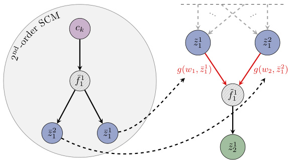
🔼 This figure shows how the model uses a second-order SCM to model temporal distribution shifts. The second-order SCM takes in the temporal domain index and outputs parameters that modify the weights of the edges in the primary SCM. This allows the model to adapt to changes in the data distribution over time. The figure visually illustrates this process by showing how a primary SCM (on the right) generates data samples for different time domains, with the edges of the SCM being shifted according to the outputs of the second-order SCM (on the left).
read the caption
Figure 3: Diagram illustrating the integration of a 2nd-order SCM for adaptive edge shifting across evolving temporal domains. On the right, the primary network G generates data samples over multiple time domains, with red arrows indicating shifted edges. On the left, the 2nd-order SCM - an auxiliary network Ĥ - takes an input domain ck ∈ C and outputs parameters to adaptively shift each edge weight wi in the base network.

🔼 This figure illustrates five different types of distribution shifts (covariate shift, prior probability shift, concept shift (X->Y), concept shift (Y->X), and other types of shifts) using Bayesian networks. Each network visually represents the relationships between features (X), labels (Y), and the context or domain (C). The figure highlights that these various shift types are inherently modeled within the prior used by the proposed Drift-Resilient TabPFN model due to the random sampling of feature and target positions, as well as edge locations within the structural causal model.
read the caption
Figure 4: Types of distribution shifts based on the definitions by Moreno-Torres et al. [51] represented as Bayesian networks as defined by Kull and Flach [52]. Here X, Y, and C denote the random variables of the features, label, and context, respectively. Note that all these types of shifts naturally arise in our prior, since we sample feature and target positions, as well as the locations of shifted edges, randomly at various positions in the synthetic datasets.
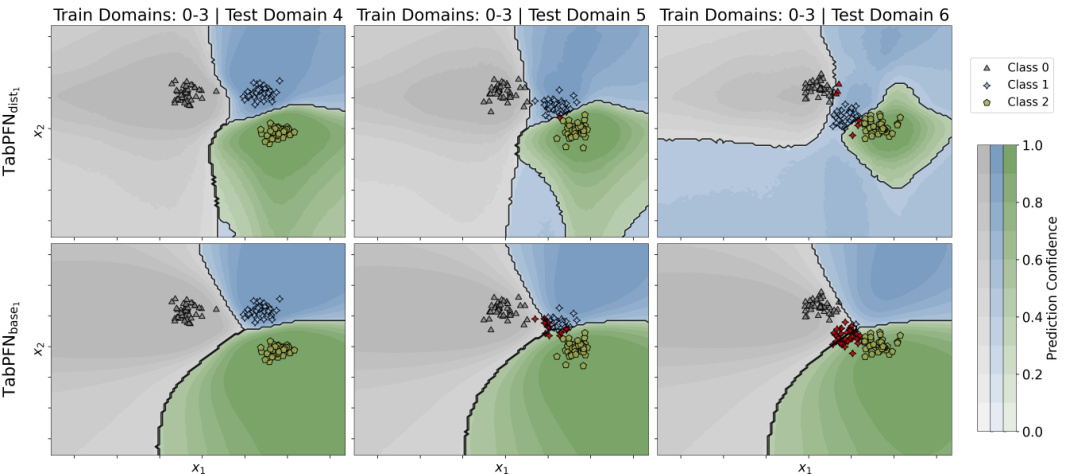
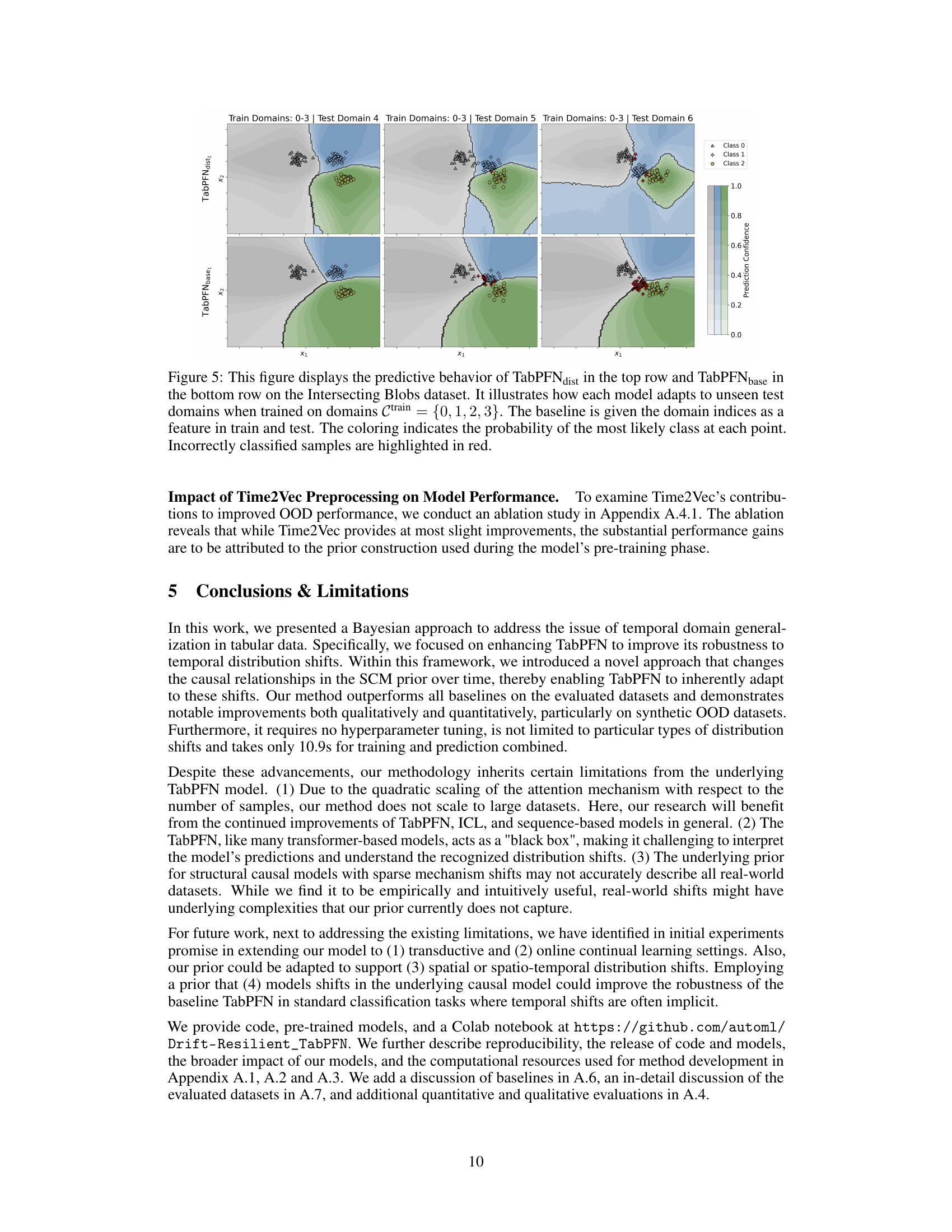
🔼 This figure compares the performance of Drift-Resilient TabPFN and the standard TabPFN on the Intersecting Blobs dataset. It shows the decision boundaries learned by each model when trained on domains 0-3 and tested on domains 4-6. The color intensity represents the prediction confidence, and misclassified points are highlighted in red. The figure illustrates how Drift-Resilient TabPFN dynamically adjusts its decision boundaries to adapt to distribution shifts in unseen data, while TabPFN maintains a relatively static boundary.
read the caption
Figure 5: This figure displays the predictive behavior of TabPFNdist in the top row and TabPFNbase in the bottom row on the Intersecting Blobs dataset. It illustrates how each model adapts to unseen test domains when trained on domains Ctrain = {0,1,2,3}. The baseline is given the domain indices as a feature in train and test. The coloring indicates the probability of the most likely class at each point. Incorrectly classified samples are highlighted in red.
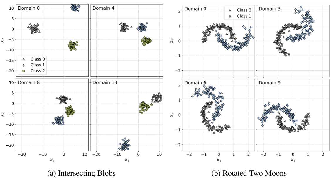
🔼 This figure visualizes the temporal shifts in two synthetic datasets, Intersecting Blobs and Rotated Two Moons, across specific domains. It provides a visual representation of how the data distributions change over time, illustrating the challenges of temporal distribution shifts in machine learning. Each sub-plot shows the data points for one specific domain, illustrating how the location and shape of the data clusters vary across different time periods.
read the caption
Figure 6: This figure shows the temporal shifts of two synthetic datasets across selected domains.

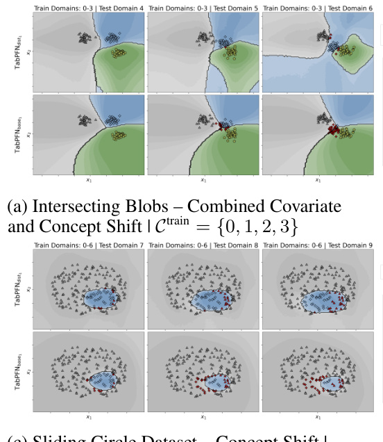
🔼 This figure compares the predictive behavior of Drift-Resilient TabPFN and the standard TabPFN model on the Intersecting Blobs dataset. It shows how each model’s decision boundary changes when presented with unseen test data (domains 4, 5, and 6), after being trained on domains 0, 1, 2, and 3. The color intensity represents the prediction confidence, with red indicating misclassified samples.
read the caption
Figure 5: This figure displays the predictive behavior of TabPFNdist in the top row and TabPFNbase in the bottom row on the Intersecting Blobs dataset. It illustrates how each model adapts to unseen test domains when trained on domains Ctrain = {0,1,2,3}. The baseline is given the domain indices as a feature in train and test. The coloring indicates the probability of the most likely class at each point. Incorrectly classified samples are highlighted in red.
🔼 This figure compares the performance of Drift-Resilient TabPFN (TabPFNdist) and the standard TabPFN (TabPFNbase) on the Intersecting Blobs dataset. It shows how well each model adapts to unseen test data (domains 4, 5, and 6) after being trained on domains 0, 1, 2, and 3. The color intensity represents the model’s prediction confidence for each class at each point, and misclassified points are highlighted in red. The comparison highlights how Drift-Resilient TabPFN adjusts its decision boundaries more effectively to handle unseen distributions shifts than the standard TabPFN.
read the caption
Figure 5: This figure displays the predictive behavior of TabPFNdist in the top row and TabPFNbase in the bottom row on the Intersecting Blobs dataset. It illustrates how each model adapts to unseen test domains when trained on domains Ctrain = {0,1,2,3}. The baseline is given the domain indices as a feature in train and test. The coloring indicates the probability of the most likely class at each point. Incorrectly classified samples are highlighted in red.

🔼 This figure compares the performance of Drift-Resilient TabPFN (TabPFNdist) and the standard TabPFN (TabPFNbase) on the Intersecting Blobs dataset. It shows how well each model extrapolates its predictions to unseen test data (domains 4, 5, and 6) after training only on domains 0, 1, 2, and 3. The color-coding represents the predicted probability of each class, highlighting misclassifications in red. The visualization demonstrates Drift-Resilient TabPFN’s superior ability to adapt its decision boundary to new, unseen data distributions.
read the caption
Figure 5: This figure displays the predictive behavior of TabPFNdist in the top row and TabPFNbase in the bottom row on the Intersecting Blobs dataset. It illustrates how each model adapts to unseen test domains when trained on domains Ctrain = {0,1,2,3}. The baseline is given the domain indices as a feature in train and test. The coloring indicates the probability of the most likely class at each point. Incorrectly classified samples are highlighted in red.

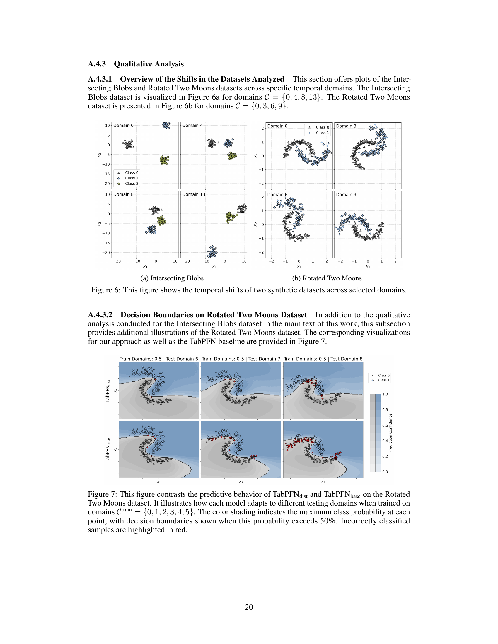
🔼 This figure compares the decision boundaries of the proposed method, DRAIN, and GI on the Rotated Two Moons dataset. The models were trained on domains 0-8 and tested on domain 9. The 50% probability contour is shown for the proposed method, while the contours for DRAIN and GI were taken from the original paper. The visualization highlights the differences in how each method adapts its decision boundary to unseen data, showcasing the superior extrapolation capabilities of the proposed approach.
read the caption
Figure 9: Comparison of our method against DRAIN [12] and GI [13] on the Rotated Two Moons dataset. The models were trained on domains C = {0,1,..., 8} and tested on domain 9. While the authors of DRAIN present different, unknown levels of the decision boundary, we present the decision boundary with 50% probability. The plots for DRAIN and GI were taken from Bai et al. [12].

🔼 This figure provides a high-level overview of the proposed Drift-Resilient TabPFN method. It illustrates the three main steps: 1) Generating synthetic datasets with time-dependent structural causal models; 2) Training a transformer model on these synthetic datasets to learn the learning algorithm itself; 3) Applying the trained model to real-world datasets, automatically detecting and adapting to distribution shifts. The figure also shows an example of the model’s ability to update decision boundaries in the presence of a distribution shift.
read the caption
Figure 1: High-level overview of our method. We train a transformer that accepts entire datasets as input to learn the learning algorithm itself by training on millions of synthetic datasets once as part of algorithm development. The trained model can be applied to arbitrary real-world datasets. In (b), X, c, and y refer to features, time domain, and label respectively. In (c), we show predictions on test domains 4 (left) and 5 (right), where we see a distribution shift. Drift-Resilient TabPFN accurately updates decision boundaries in this example.
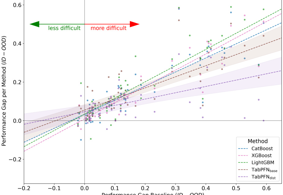
🔼 This figure shows a comparative analysis of how different models’ performance changes in relation to the difficulty of the dataset regarding out-of-distribution (OOD) shifts. The x-axis shows dataset difficulty, measured as the difference in performance between in-distribution and out-of-distribution. The y-axis shows how much each model’s performance drops from ID to OOD. The plot shows that Drift-Resilient TabPFN is the most resilient to increasing dataset difficulty, maintaining performance better than baselines.
read the caption
Figure 11: This figure illustrates a comparative analysis of the resilience of the listed methods to out-of-distribution (OOD) difficulty across multiple datasets and splits. The x-axis captures the difficulty of each dataset split, while the y-axis measures the performance drop of a method compared to in-distribution (ID) performance. Individual methods are represented by scatter points and their corresponding linear regression lines, with shaded regions indicating the 95% confidence intervals for TabPFN methods. Directional arrows signify increasing or decreasing dataset difficulty. Flatter regression slopes indicate models that are more resilient to increases in dataset difficulty due to distribution shifts.

🔼 This figure compares the performance of Drift-Resilient TabPFN and the standard TabPFN on the Intersecting Blobs dataset when varying the number of training domains (from 2 to 9). The evaluation metric (Accuracy, F1 Score, ROC AUC, and ECE) are shown on test domain 9 in separate subfigures. The results highlight Drift-Resilient TabPFN’s ability to extrapolate effectively with a smaller number of training domains compared to TabPFN.
read the caption
Figure 12: This figure shows the performance of Drift-Resilient TabPFN and the baseline TabPFN on the Intersecting Blobs dataset. Thereby, we always test on domain Ctest = {9} and gradually increase on the x-axis the number of training domains starting with Ctrain = {0, 1} up to Ctrain = {0,1,...,8}. The results show that Drift-Resilient TabPFN achieves effective extrapolation with as few as four training domains, while TabPFN-base needs significantly more to reach similar performance.

🔼 This figure illustrates how the model incorporates temporal information into its handling of distribution shifts by using a secondary SCM (2nd-order SCM). This secondary SCM takes a temporal domain indicator as input and outputs parameters that dynamically adjust the weights of the edges within the main SCM. These adjusted weights then affect the data generation process, enabling the model to adapt to evolving temporal distribution shifts.
read the caption
Figure 3: Diagram illustrating the integration of a 2nd-order SCM for adaptive edge shifting across evolving temporal domains. On the right, the primary network G generates data samples over multiple time domains, with red arrows indicating shifted edges. On the left, the 2nd-order SCM - an auxiliary network Ĥ - takes an input domain ck ∈ C and outputs parameters to adaptively shift each edge weight wi in the base network.
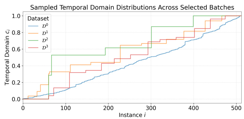
🔼 This figure shows the distribution of temporal domains across four different datasets. Each line represents a different dataset, and the y-axis shows the cumulative proportion of instances from each domain up to a given instance index (x-axis). The figure highlights the variability in domain size and the presence of gaps, reflecting the irregularities in real-world data.
read the caption
Figure 14: Share of temporal domains in exemplary datasets prior seen up to any instance i. The figure illustrates the range and structure of the sampled temporal domains ck ∈ C across four representative datasets. It highlights variations in domain size and demonstrates the presence of arbitrary gaps, simulating irregularities in data sampling.

🔼 This figure shows three example functions generated by the second-order SCM (H) used in the Drift-Resilient TabPFN model. The x-axis represents the temporal domain (cᵢ), and the y-axis represents the sampled function values (hⱼ(cᵢ)). Each function (h₀(cᵢ), h₁(cᵢ), h₂(cᵢ)) shows a unique curve demonstrating the variation in edge weight changes over time that the 2nd-order SCM generates. This helps to model complex distribution shifts.
read the caption
Figure 15: This figure presents three exemplary functions sampled from nodes within the network of a 2nd-order SCM H. In the plot, the x-axis represents the input temporal domain cᵢ ∈ C, while the y-axis displays the corresponding node activation.

🔼 This figure provides a high-level overview of the proposed Drift-Resilient TabPFN method. It illustrates the three main stages: (a) Generating synthetic datasets with temporal distribution shifts using structural causal models, (b) Training a transformer model on these datasets to learn the prediction algorithm itself, and (c) Applying the trained model to real-world datasets to make predictions in a single forward pass, automatically handling distribution shifts. The figure also includes detailed descriptions of the inputs and outputs of the model.
read the caption
Figure 1: High-level overview of our method. We train a transformer that accepts entire datasets as input to learn the learning algorithm itself by training on millions of synthetic datasets once as part of algorithm development. The trained model can be applied to arbitrary real-world datasets. In (b), X, c, and y refer to features, time domain, and label respectively. In (c), we show predictions on test domains 4 (left) and 5 (right), where we see a distribution shift. Drift-Resilient TabPFN accurately updates decision boundaries in this example.
More on tables

🔼 This table presents a comparison of the proposed Drift-Resilient TabPFN model against several baseline models on 18 datasets (8 synthetic, 10 real-world). Performance metrics (Accuracy, F1-score, ROC AUC, and ECE) are reported for both in-distribution (ID) and out-of-distribution (OOD) data. The results are averaged over three runs and include 95% confidence intervals. The best-performing model for each metric is highlighted in bold.
read the caption
Table 1: Comparison of Drift-Resilient TabPFN with various baselines and settings across the subsets of synthetic and real-world datasets. Metrics include accuracy, F1, ROC, and ECE for both in-distribution (ID) and out-of-distribution (OOD) data, averaged over three initializations and reported with 95% confidence intervals. The best mean of each metric within a dataset subset is marked in bold. Metric arrows indicate optimization direction.

🔼 This table presents a comprehensive comparison of the proposed Drift-Resilient TabPFN model against several baseline methods across a diverse set of 18 datasets (8 synthetic, 10 real-world). The performance is evaluated using four key metrics: Accuracy, F1-score, ROC AUC, and ECE. Results are shown for both in-distribution (ID) and out-of-distribution (OOD) data, reflecting the model’s ability to generalize beyond the training data. The table highlights the best-performing model for each metric in each dataset subset.
read the caption
Table 1: Comparison of Drift-Resilient TabPFN with various baselines and settings across the subsets of synthetic and real-world datasets. Metrics include accuracy, F1, ROC, and ECE for both in-distribution (ID) and out-of-distribution (OOD) data, averaged over three initializations and reported with 95% confidence intervals. The best mean of each metric within a dataset subset is marked in bold. Metric arrows indicate optimization direction.

🔼 This table compares the out-of-distribution (OOD) accuracy of Drift-Resilient TabPFN against two state-of-the-art methods, DRAIN and GI, on the Rotated Two Moons dataset. It shows the mean OOD accuracy and its standard deviation for each method. The results for DRAIN and GI are taken from the referenced paper by Bai et al. [12].
read the caption
Table 4: Comparison of Drift-Resilient TabPFN against DRAIN and GI on the Rotated Two Moons dataset. The metric reported is the mean out-of-distribution (OOD) accuracy along with the standard deviation. Results for DRAIN and GI are taken from Bai et al. [12].

🔼 This table presents a comprehensive comparison of the proposed Drift-Resilient TabPFN model against various baseline methods across 18 datasets (8 synthetic and 10 real-world). For each dataset subset (synthetic and real-world), it shows the performance of different models and variations using four evaluation metrics: Accuracy, F1-score, ROC AUC, and ECE. The results are averaged over three different initializations and presented with 95% confidence intervals. The best-performing model for each metric in each dataset subset is highlighted in bold.
read the caption
Table 1: Comparison of Drift-Resilient TabPFN with various baselines and settings across the subsets of synthetic and real-world datasets. Metrics include accuracy, F1, ROC, and ECE for both in-distribution (ID) and out-of-distribution (OOD) data, averaged over three initializations and reported with 95% confidence intervals. The best mean of each metric within a dataset subset is marked in bold. Metric arrows indicate optimization direction.

🔼 This table presents a comprehensive comparison of the proposed Drift-Resilient TabPFN model against several baseline methods across various datasets. It shows the accuracy, F1 score, ROC AUC, and Expected Calibration Error (ECE) for both in-distribution (ID) and out-of-distribution (OOD) data. The results are averaged over multiple runs to provide confidence intervals, and the best-performing methods are highlighted for each metric. The table helps to quantify the performance improvements of the proposed method, particularly in handling out-of-distribution data.
read the caption
Table 1: Comparison of Drift-Resilient TabPFN with various baselines and settings across the subsets of synthetic and real-world datasets. Metrics include accuracy, F1, ROC, and ECE for both in-distribution (ID) and out-of-distribution (OOD) data, averaged over three initializations and reported with 95% confidence intervals. The best mean of each metric within a dataset subset is marked in bold. Metric arrows indicate optimization direction.
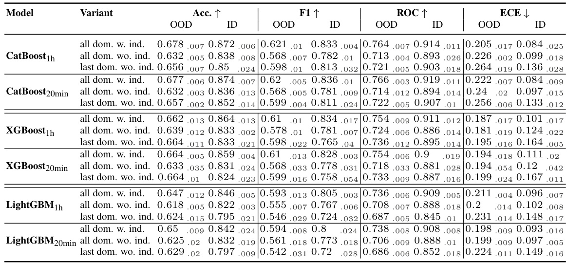
🔼 This table presents a comparison of the proposed Drift-Resilient TabPFN model against several baseline methods across a range of synthetic and real-world datasets. It shows the performance of each model in terms of accuracy, F1 score, ROC AUC, and Expected Calibration Error (ECE) for both in-distribution (ID) and out-of-distribution (OOD) settings. The results are averaged over three independent runs and include 95% confidence intervals. The best performing model for each metric in each dataset subset is highlighted in bold.
read the caption
Table 1: Comparison of Drift-Resilient TabPFN with various baselines and settings across the subsets of synthetic and real-world datasets. Metrics include accuracy, F1, ROC, and ECE for both in-distribution (ID) and out-of-distribution (OOD) data, averaged over three initializations and reported with 95% confidence intervals. The best mean of each metric within a dataset subset is marked in bold. Metric arrows indicate optimization direction.

🔼 This table presents a quantitative comparison of the proposed Drift-Resilient TabPFN model against several baseline methods across a range of synthetic and real-world datasets. The performance is evaluated using multiple metrics: accuracy, F1-score, ROC AUC, and Expected Calibration Error (ECE). The results are shown for both in-distribution (ID) and out-of-distribution (OOD) data, which helps to assess the model’s generalization ability to unseen data. The best performing model for each metric in each dataset subset is highlighted in bold, and the overall trend of optimization for each metric (improvement or reduction) is indicated by arrows.
read the caption
Table 1: Comparison of Drift-Resilient TabPFN with various baselines and settings across the subsets of synthetic and real-world datasets. Metrics include accuracy, F1, ROC, and ECE for both in-distribution (ID) and out-of-distribution (OOD) data, averaged over three initializations and reported with 95% confidence intervals. The best mean of each metric within a dataset subset is marked in bold. Metric arrows indicate optimization direction.
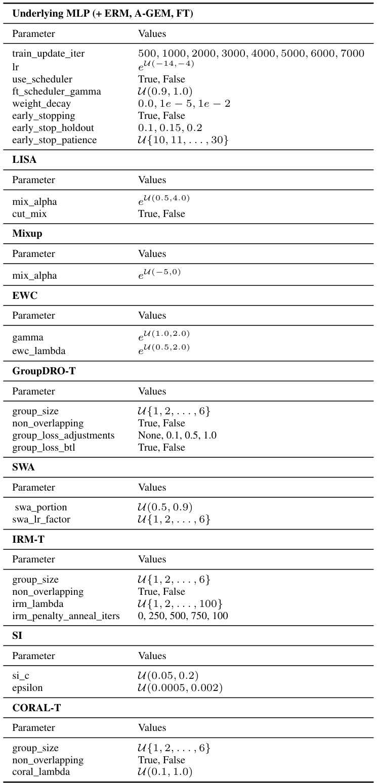
🔼 This table presents a detailed comparison of the proposed Drift-Resilient TabPFN model against several baseline methods across various datasets. It shows performance metrics (accuracy, F1-score, ROC AUC, and ECE) for both in-distribution (ID) and out-of-distribution (OOD) data, providing a comprehensive evaluation of the model’s robustness to distribution shifts. The best performing model for each metric in each dataset subset is highlighted in bold.
read the caption
Table 1: Comparison of Drift-Resilient TabPFN with various baselines and settings across the subsets of synthetic and real-world datasets. Metrics include accuracy, F1, ROC, and ECE for both in-distribution (ID) and out-of-distribution (OOD) data, averaged over three initializations and reported with 95% confidence intervals. The best mean of each metric within a dataset subset is marked in bold. Metric arrows indicate optimization direction.

🔼 This table presents a comprehensive comparison of the proposed Drift-Resilient TabPFN model against several baseline methods across 18 datasets (8 synthetic, 10 real-world). It shows the performance of each model (including different configurations) in terms of accuracy, F1-score, ROC AUC, and Expected Calibration Error (ECE), both for in-distribution (ID) and out-of-distribution (OOD) data. The best-performing model for each metric is highlighted in bold. The table demonstrates the superior performance of Drift-Resilient TabPFN, especially for OOD data, and provides quantitative support for the claims made in the paper.
read the caption
Table 1: Comparison of Drift-Resilient TabPFN with various baselines and settings across the subsets of synthetic and real-world datasets. Metrics include accuracy, F1, ROC, and ECE for both in-distribution (ID) and out-of-distribution (OOD) data, averaged over three initializations and reported with 95% confidence intervals. The best mean of each metric within a dataset subset is marked in bold. Metric arrows indicate optimization direction.

🔼 This table presents a quantitative comparison of the proposed Drift-Resilient TabPFN model against several baseline methods across 18 datasets (8 synthetic and 10 real-world). For each dataset, the table shows the performance of different model variants and baselines in terms of accuracy, F1-score, ROC AUC, and Expected Calibration Error (ECE) for both in-distribution (ID) and out-of-distribution (OOD) data. The best performing model for each metric is highlighted in bold. The results are averaged across three separate model initializations and include 95% confidence intervals. The table also indicates the direction of optimization for each metric (improvement indicated by an upward-pointing arrow).
read the caption
Table 1: Comparison of Drift-Resilient TabPFN with various baselines and settings across the subsets of synthetic and real-world datasets. Metrics include accuracy, F1, ROC, and ECE for both in-distribution (ID) and out-of-distribution (OOD) data, averaged over three initializations and reported with 95% confidence intervals. The best mean of each metric within a dataset subset is marked in bold. Metric arrows indicate optimization direction.
Full paper#
