TL;DR#
Current Tensor-based Multi-view Subspace Clustering (TMSC) methods suffer from high computational complexity, inaccurate subspace representation, and under-penalization of noise. These limitations hinder their application to large-scale datasets and noisy data, necessitating improvements in both efficiency and accuracy.
The proposed Scalable TMSC framework with Triple Information Enhancement (STONE) tackles these issues. It uses an enhanced anchor dictionary learning mechanism to reduce complexity and improve robustness. Further, it incorporates an anchor hypergraph Laplacian regularizer to accurately capture data geometry and employs an improved hyperbolic tangent function to precisely approximate tensor rank, effectively distinguishing significant variations in singular values. Extensive experiments demonstrate STONE’s superior performance in both effectiveness and efficiency compared to state-of-the-art methods.
Key Takeaways#
Why does it matter?#
This paper is crucial for researchers in multi-view subspace clustering due to its enhanced scalability and accuracy. It offers a novel approach to address limitations of existing methods, opening avenues for improving efficiency and handling noisy data. The proposed framework and its innovative techniques directly impact the field’s advancement, providing a strong foundation for future research in large-scale multi-view data analysis.
Visual Insights#

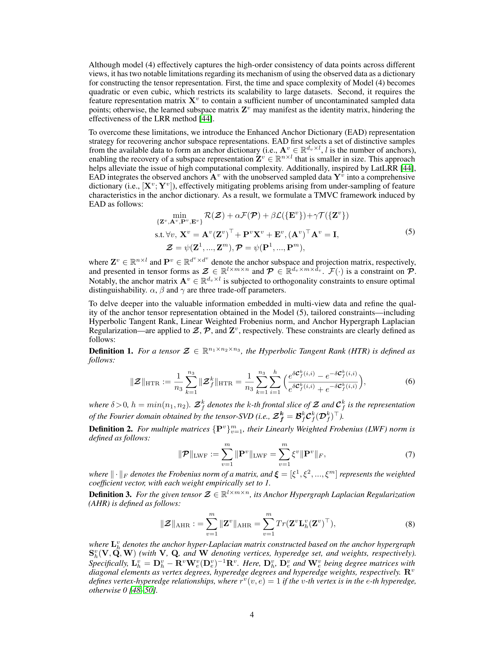
🔼 This figure illustrates the Enhanced Anchor Dictionary (EAD) representation strategy used in the STONE model. The EAD method is designed to improve the efficiency and robustness of subspace representation learning, particularly when dealing with limited or noisy data. Instead of directly using the observed data as a dictionary, EAD selects a subset of data points as anchors. These anchors, along with additional latent data points, construct a smaller, more efficient dictionary that is less prone to the issues associated with using the full dataset directly. The figure visually shows how the anchor dictionary (Av), the subspace representation (Zv), the projection matrix (Pv), the observed data (Xv), and the reconstruction error (Ev) interact to form the subspace representation of view v in the STONE framework.
read the caption
Figure 1: Schematic of Enhanced Anchor Dictionary Representation (EAD).
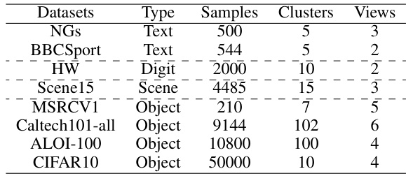
🔼 This table presents the characteristics of eight datasets used in the paper’s experiments. For each dataset, it lists the type of data (text, digit, scene, or object), the number of samples, the number of clusters, and the number of views.
read the caption
Table 1: Overview of Statistical Features for Eight Datasets.
In-depth insights#
Triple Info Enhance#
The concept of “Triple Info Enhance” suggests a multi-pronged approach to improving data representation and analysis. It likely involves enhancing three distinct aspects of information within a dataset. This approach could focus on improving the quality of the data by reducing noise or handling missing values, enhancing the representation of the data, perhaps using a higher-order representation like tensors instead of matrices, and improving the integration of information from multiple sources or views, perhaps via a more sophisticated fusion strategy. By combining these three enhancements, “Triple Info Enhance” aims to achieve a more robust and accurate data analysis, leading to better results in tasks like clustering, classification or dimensionality reduction. The “triple” aspect highlights the synergistic effect of combined improvements, implying that each enhancement reinforces the others, producing a more significant overall improvement than if each were applied individually. This strategy likely addresses common limitations of single-view or lower-order techniques, leading to a more powerful and scalable framework for complex data analysis.
Anchor Dictionary#
The concept of an ‘Anchor Dictionary’ in the context of multi-view subspace clustering is a significant innovation addressing limitations of traditional methods. Instead of using the entire observed data as a dictionary for subspace representation, which can be computationally expensive and sensitive to noise or incomplete data, an anchor dictionary leverages a carefully selected subset of data points, the anchors, to represent the entire dataset’s subspace structure. This approach offers several key advantages: First, it significantly reduces computational complexity, making the method scalable to larger datasets. Second, by using a curated set of anchors, it enhances the robustness of subspace representation, making it more resilient to noisy or incomplete input. The selection of anchors, a crucial step in this process, requires careful consideration and may use techniques to ensure representativeness and avoid redundancy. Furthermore, the use of an anchor dictionary may be combined with regularization techniques, such as an anchor hypergraph Laplacian, to further refine subspace representation and capture intrinsic data geometry. This enhances the overall accuracy of the model and strengthens its ability to obtain meaningful clustering results. Ultimately, the anchor dictionary approach, by selecting a representative subset of data points, is a powerful tool for enhancing both efficiency and effectiveness in multi-view subspace clustering.
HTR Tensor Rank#
The proposed Hyperbolic Tangent Rank (HTR) offers a novel approach to tensor rank approximation, improving upon existing methods like Tensor Nuclear Norm (TNN). HTR’s non-convex nature allows it to distinguish between singular values of varying significance, unlike TNN, which treats all singular values equally. This is crucial because larger singular values often represent essential data features, while smaller ones may correspond to noise. By applying variable penalties, HTR effectively captures significant variations in singular values, leading to a more robust and accurate tensor representation. This improved representation is particularly beneficial for multi-view subspace clustering, enhancing the algorithm’s overall effectiveness and efficiency by enabling the model to better differentiate between salient data features and noise.
Scalable TMSC#
The concept of “Scalable TMSC” (Tensor-based Multi-view Subspace Clustering) points towards a crucial advancement in the field of multi-view data analysis. Traditional TMSC methods often struggle with high computational complexity, limiting their applicability to large datasets. A scalable approach directly addresses this limitation, enabling the processing of massive datasets that were previously intractable. This scalability is likely achieved through algorithmic improvements, potentially involving techniques like efficient tensor decompositions, randomized algorithms, or clever data partitioning strategies. The core idea is to maintain the accuracy and effectiveness of TMSC while significantly reducing the computational burden, making it practical for real-world applications involving large-scale multi-view data, such as those encountered in image recognition, social network analysis, or bioinformatics. Further research in this area might focus on exploring the trade-offs between scalability and accuracy, developing more robust methods that are resistant to noise and outliers in large datasets, and potentially investigating parallel or distributed implementations for further performance enhancement.
Future Enhancements#
Future enhancements for the described multi-view subspace clustering framework could involve exploring more sophisticated anchor selection strategies to further improve efficiency and robustness. Investigating alternative low-rank regularizers beyond the hyperbolic tangent rank could reveal additional improvements in capturing subtle variations in singular values. The framework’s scalability could be further enhanced by incorporating distributed or parallel processing techniques, allowing for efficient handling of even larger datasets. Incorporating uncertainty modeling into the framework would enhance its ability to manage noisy or incomplete data. Finally, exploring the applications of the framework to a wider array of multi-view datasets, such as those with heterogeneous data types or significantly varying numbers of views, would be a valuable area of future investigation. Extending the anchor hypergraph to incorporate temporal information would enable analysis of time-evolving multi-view data. Combining the framework with deep learning techniques may also yield significant performance gains, but would require careful investigation.
More visual insights#
More on figures

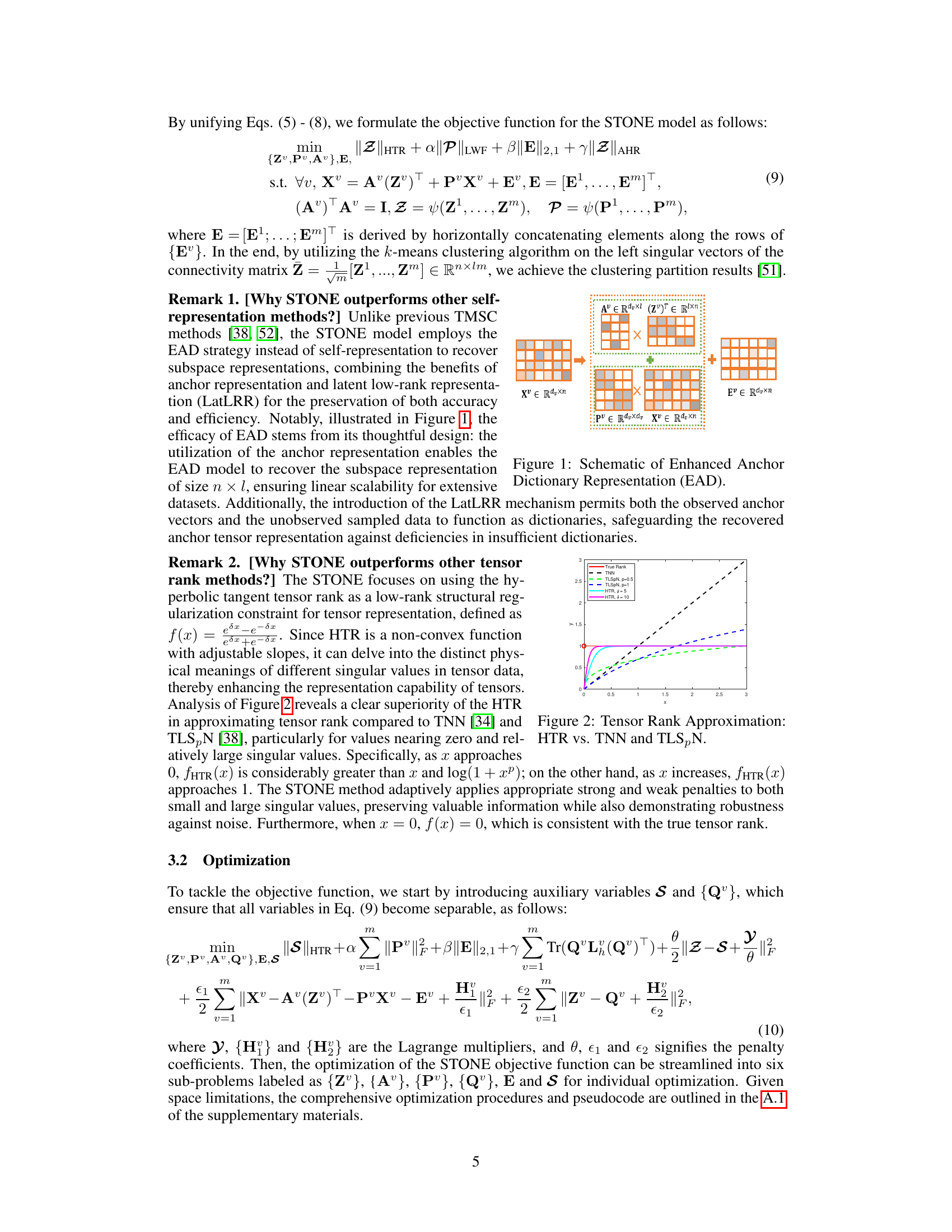
🔼 This figure compares the performance of the proposed Hyperbolic Tangent Rank (HTR) approximation to existing tensor rank approximations, namely Tensor Nuclear Norm (TNN) and Truncated Logarithmic Schatten-p Norm (TLSPN). It shows that HTR more precisely approximates the tensor rank across a range of values, particularly for those close to zero and larger values. This more accurate approximation allows HTR to better distinguish between significant variations and noise within the singular values of the tensor data.
read the caption
Figure 2: Tensor Rank Approximation: HTR vs. TNN and TLSN.

🔼 This figure demonstrates the effect of varying the parameter δ (delta) in the STONE model on the clustering performance across different datasets. The x-axis represents the values of δ, and the y-axis represents the clustering performance metrics (ACC and NMI). The different curves in the figure represent the results obtained for different datasets (NGs, HW, and MSRCV1). It shows how the choice of δ impacts the clustering results, revealing that an optimal δ value exists for each dataset, maximizing the effectiveness of the STONE model’s capability to capture non-linear correlations.
read the caption
Figure 3: Impact of Parameter δ on the STONE Model.

🔼 This figure displays the impact of varying the number of anchors on the STONE model’s performance across three different datasets (NGs, HW, and MSRCV1). The x-axis represents the number of anchors (multiples of a base number ‘c’), and the y-axis shows the clustering accuracy (ACC) and Normalized Mutual Information (NMI). The results indicate that choosing a smaller number of discriminative anchors is better than using a larger number of non-discriminative anchors, and the optimal performance is achieved with ‘c’ or ‘2c’ anchors. This demonstrates the effectiveness of the anchor selection strategy in STONE.
read the caption
Figure 4: The Influence of Anchor Quantity on STONE Model Performance.

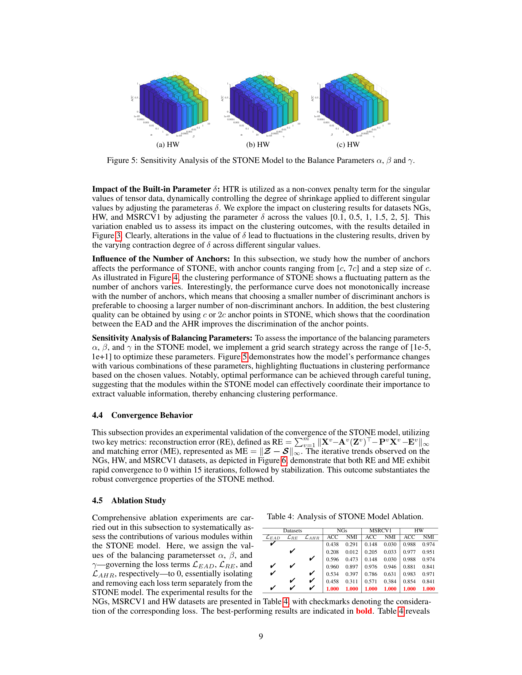
🔼 This figure presents a sensitivity analysis of the STONE model’s performance concerning its three balancing parameters: α, β, and γ. The plots show how the accuracy (ACC) of the model changes as these parameters are varied across different values, providing insights into their relative importance and optimal ranges for achieving the best clustering performance. Each subplot represents the result for a specific dataset (HW in this case), showing the interplay between α and β at various values of γ, allowing for a comprehensive understanding of the parameters’ impact on the model’s efficacy.
read the caption
Figure 5: Sensitivity Analysis of the STONE Model to the Balance Parameters α, β and γ.

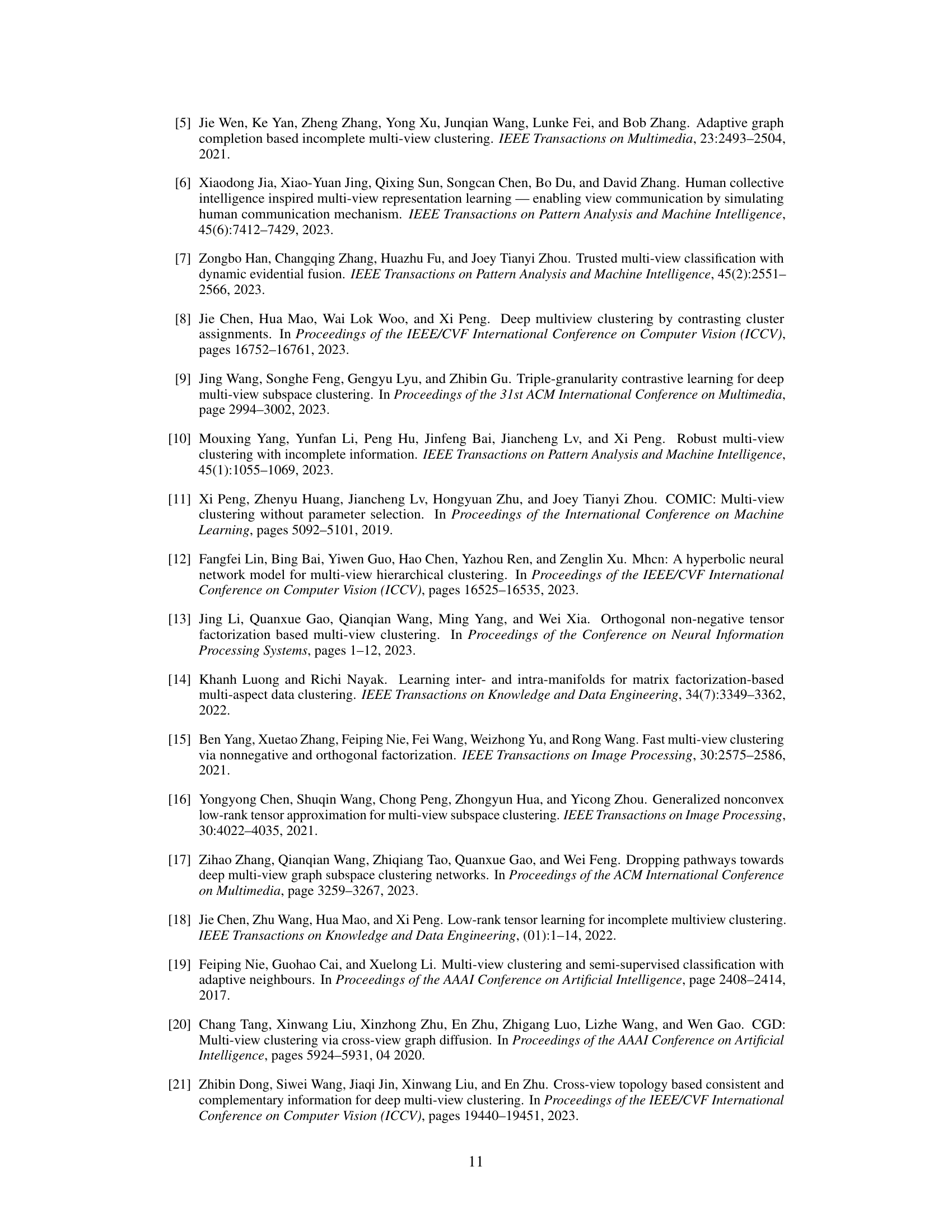
🔼 This figure displays the convergence behavior of the STONE model’s optimization algorithm across three different datasets: NGs, HW, and MSRCV1. The plots show the reconstruction error (RE) and matching error (ME) over a series of iterations. The rapid decrease and subsequent stabilization of both RE and ME indicate the algorithm’s efficient convergence to a solution, demonstrating its robust behavior across varied datasets.
read the caption
Figure 6: Convergence Curves of STONE on Three Datasets.

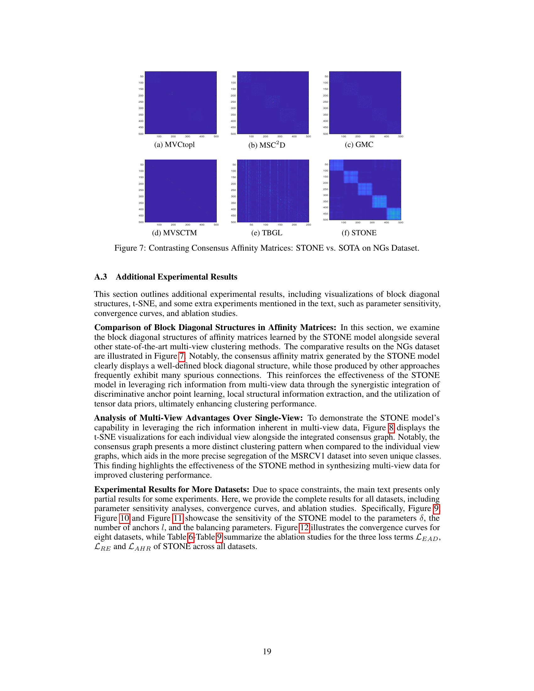
🔼 The figure compares the consensus affinity matrices generated by different multi-view clustering methods, including MVCtopl, MSC2D, GMC, MVSCTM, TBGL, and the proposed STONE model. The visualization highlights how the STONE model produces a more well-defined block-diagonal structure compared to other methods, indicating a more effective clustering of the data points. This showcases the superiority of STONE in learning high-order correlations and local geometric structures within the data.
read the caption
Figure 7: Contrasting Consensus Affinity Matrices: STONE vs. SOTA on NGs Dataset.

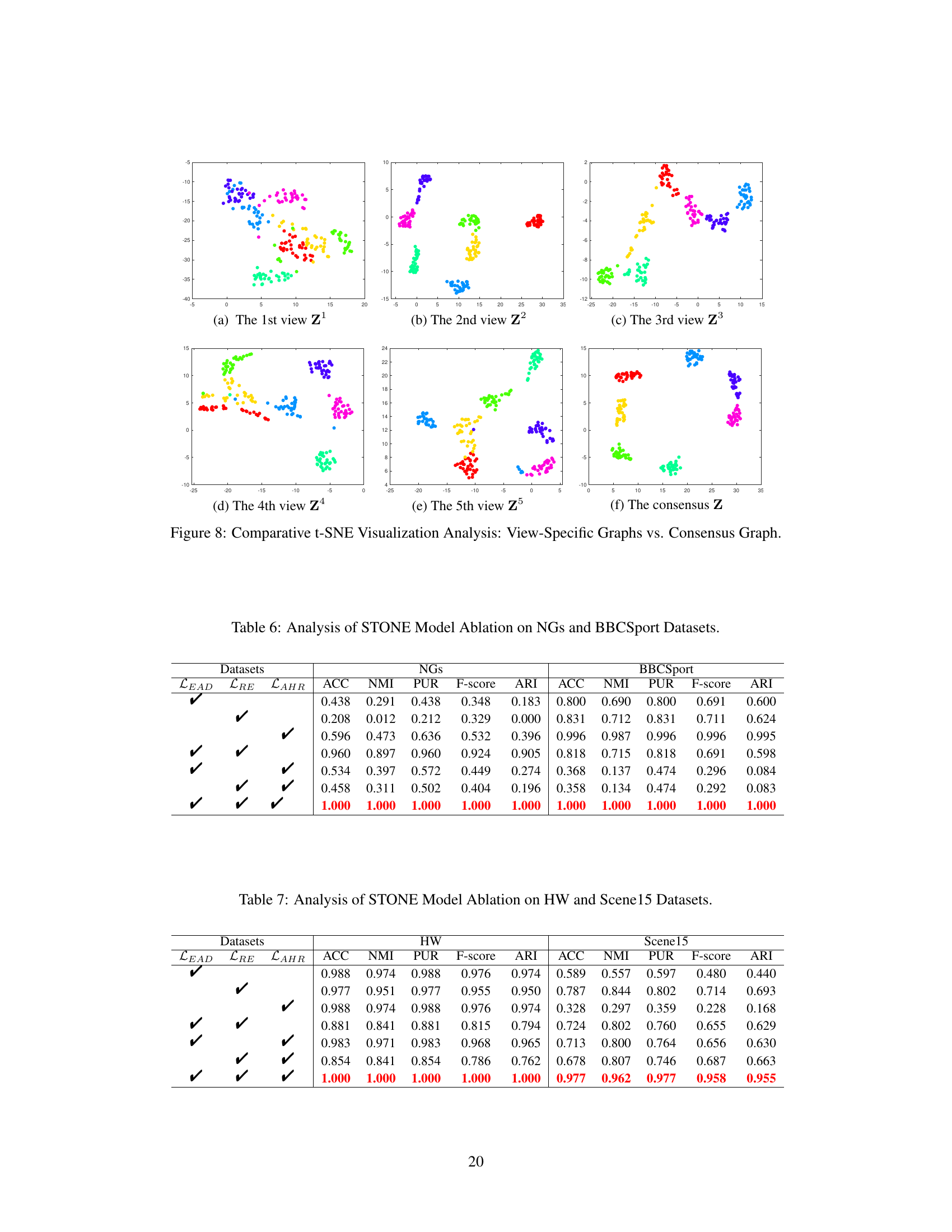
🔼 This figure visualizes the results of t-SNE dimensionality reduction applied to the MSRCV1 dataset. It shows separate t-SNE plots for each of the five individual views (a-e), as well as a t-SNE plot (f) of the consensus representation learned by the STONE model which integrates information across all views. The visualization aims to demonstrate that the consensus representation obtained by the STONE model provides a more distinct separation of clusters compared to the individual views, highlighting the benefits of multi-view integration in improving clustering performance.
read the caption
Figure 8: Comparative t-SNE Visualization Analysis: View-Specific Graphs vs. Consensus Graph.
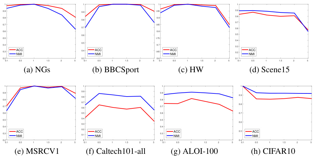
🔼 This figure displays the impact of the built-in parameter δ on the performance of the STONE model across eight datasets. The parameter δ controls the degree of shrinkage applied to different singular values, affecting how well the model distinguishes between significant variations and noise within the tensor data. The graphs show that changes in the value of δ lead to fluctuations in clustering performance (ACC and NMI), demonstrating its sensitivity and the importance of careful tuning for optimal results. The performance varies for each dataset, highlighting the data-dependent nature of this parameter and the need for careful selection.
read the caption
Figure 9: Impact of Parameter δ on the STONE Model on Eight Datasets.

🔼 This figure displays the impact of the built-in parameter δ on the STONE model’s performance across eight different datasets. The parameter δ dynamically controls the degree of shrinkage applied to different singular values of tensor data. The x-axis represents the various values of δ tested, while the y-axis shows the corresponding ACC and NMI values. The plots illustrate how different values of δ influence clustering performance (ACC and NMI) for each dataset. This analysis helps in understanding how the non-convex penalty term (HTR) works and its sensitivity to different δ values.
read the caption
Figure 9: Impact of Parameter δ on the STONE Model on Eight Datasets.
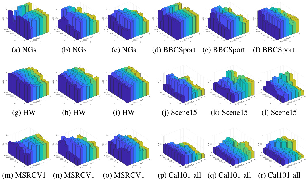
🔼 This figure displays a sensitivity analysis of the STONE model’s performance to its three balancing parameters (α, β, and γ) across eight different datasets. Each subfigure shows a 3D surface plot illustrating the relationship between the three parameters and the resulting accuracy (ACC) achieved on a specific dataset. The plots help to visualize the optimal parameter ranges for achieving high clustering accuracy and highlight the interplay between the parameters in influencing performance.
read the caption
Figure 11: Sensitivity Analysis of the STONE Model to Parameters α, β and γ on Eight Datasets.

🔼 This figure displays a sensitivity analysis of the STONE model’s performance across eight datasets with respect to variations in three balancing parameters (α, β, and γ). Each subfigure represents a different dataset, showing how changes in the parameters affect the accuracy (ACC) and normalized mutual information (NMI) scores. The 3D plots visualize the parameter space, providing insights into the model’s robustness and optimal parameter ranges for different datasets.
read the caption
Figure 11: Sensitivity Analysis of the STONE Model to Parameters α, β and γ on Eight Datasets.

🔼 This figure displays the convergence behavior of the STONE model’s optimization process on three datasets: NGs, HW, and MSRCV1. The plots track two key metrics: reconstruction error (RE) and matching error (ME) over a series of iterations. The rapid decrease and eventual stabilization of both RE and ME demonstrate the model’s efficient and robust convergence to a solution.
read the caption
Figure 6: Convergence Curves of STONE on Three Datasets.
More on tables

🔼 This table compares the computational efficiency of different multi-view clustering methods on datasets with more than 4,000 samples. The efficiency is measured in terms of the running time (in seconds) for each method on four different datasets: Scene15, ALOI-100, Caltech101-all, and CIFAR10. The results show that the proposed STONE method significantly outperforms other state-of-the-art methods in terms of computational efficiency.
read the caption
Table 3: Efficiency Comparison of Different Methods on Datasets with over 4,000 Samples.
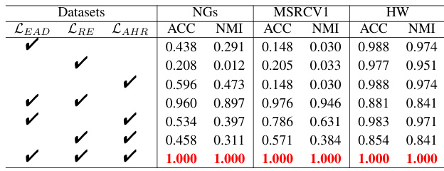
🔼 This table presents the results of ablation studies performed on the Caltech101-all and CIFAR10 datasets. The studies evaluated the impact of removing individual loss terms (LEAD, LRE, LAHR) from the STONE model’s objective function. Each row represents a configuration, showing whether each loss term was included (√) or excluded ( ). The ACC, NMI, PUR, F-score, and ARI metrics are then reported for each configuration, demonstrating the relative importance of each loss term to the overall performance of the STONE model. The last row shows the full model’s performance.
read the caption
Table 9: Analysis of STONE Model Ablation on Caltech101-all and CIFAR10 Datasets.

🔼 This table presents a detailed comparison of the clustering performance of the proposed STONE model against ten other state-of-the-art (SOTA) methods across eight different datasets. The performance is evaluated using five common metrics: Accuracy (ACC), Normalized Mutual Information (NMI), Purity (PUR), F-score, and Adjusted Rand Index (ARI). Higher values indicate better clustering performance. The table shows the mean and standard deviation of each metric across multiple runs, providing a comprehensive statistical analysis of the results. The results demonstrate the superior clustering accuracy and robustness of the STONE model compared to existing methods.
read the caption
Table 2: Clustering Performance Comparison Across Eight Datasets (Mean ± Standard Deviation).

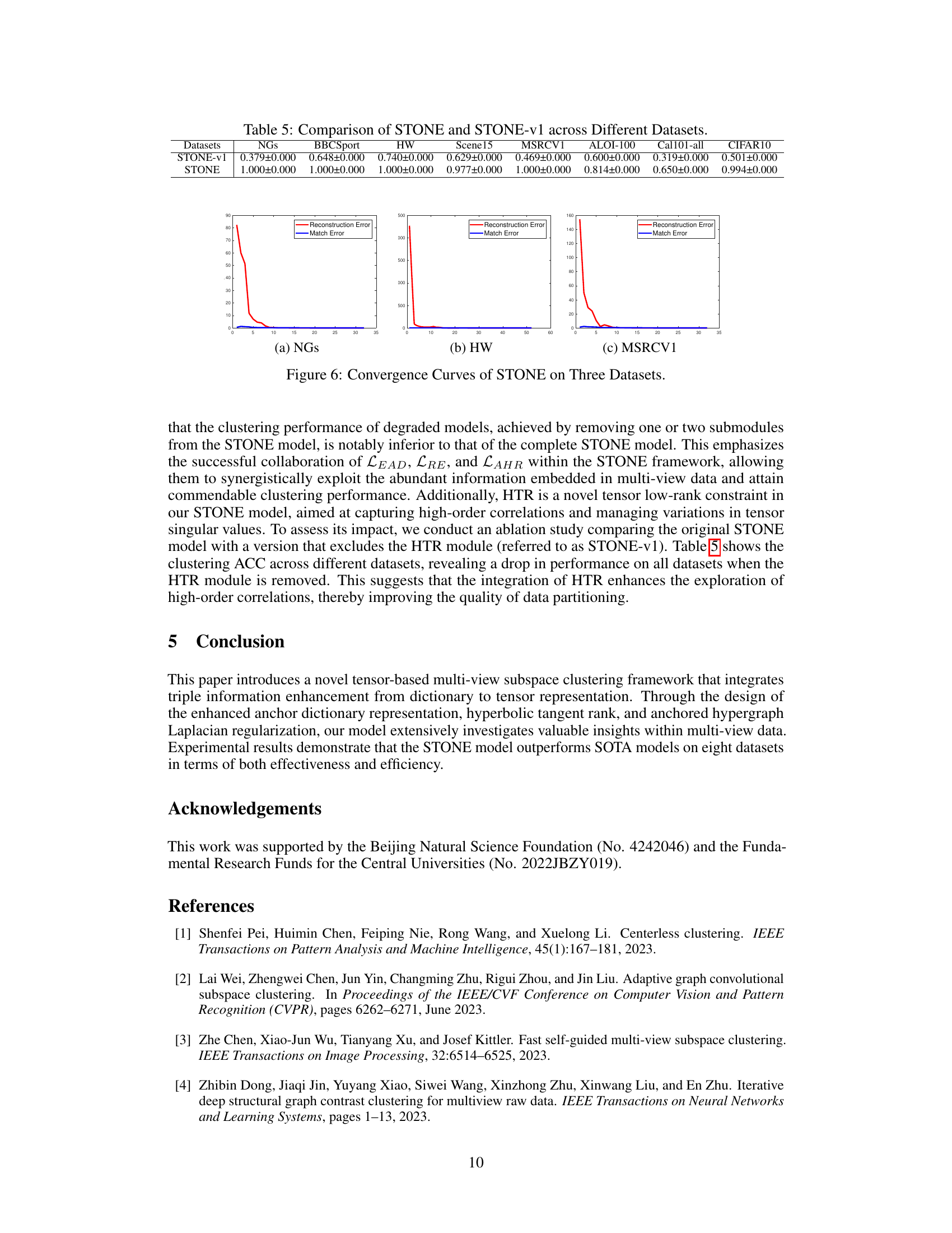
🔼 This table presents the ablation study results for the STONE model on Caltech101-all and CIFAR10 datasets. It shows the clustering performance (ACC, NMI, PUR, F-score, ARI) when different components of the model (LEAD, LRE, LAHR) are removed. The results demonstrate the contribution of each component to the overall performance. The checkmarks indicate which components were included in the experiment. The best performing results are shown in bold.
read the caption
Table 9: Analysis of STONE Model Ablation on Caltech101-all and CIFAR10 Datasets.

🔼 This table presents the ablation study results on MSRCV1 and ALOI-100 datasets. It shows the clustering performance (ACC, NMI, PUR, F-score, ARI) when different components (LEAD, LRE, LAHR) of the proposed STONE model are removed. The results demonstrate the impact of each component on the overall performance, highlighting their contribution to achieving high accuracy.
read the caption
Table 8: Analysis of STONE Model Ablation on MSRCV1 and ALOI-100 Datasets.

🔼 This table presents the ablation study results on the Caltech101-all and CIFAR10 datasets. It shows the clustering performance (ACC, NMI, PUR, F-score, ARI) when different combinations of the three loss terms (LEAD, LRE, LAHR) are included in the STONE model. The results demonstrate the contribution of each loss term to the overall performance, highlighting the importance of integrating all three for optimal results.
read the caption
Table 9: Analysis of STONE Model Ablation on Caltech101-all and CIFAR10 Datasets.
Full paper#
