On Causal Discovery in the Presence of Deterministic Relations

pfvcsgFrJ6

Loka Li et el.

TL;DR
#

Many causal discovery methods assume independent noise, which is often violated in real-world scenarios exhibiting deterministic relations. This leads to challenges for constraint-based methods that rely on the faithfulness assumption. Score-based methods using exact search can handle determinism better but are computationally expensive.

The paper proposes a novel method, Determinism-aware Greedy Equivalent Search (DGES), to address these issues. DGES uses a three-phase approach: (1) identifying minimal deterministic clusters, (2) running a modified Greedy Equivalent Search (GES) globally, and (3) performing exact search only on deterministic clusters and their neighbors. DGES is shown to be more efficient and accurate than existing methods, accommodating various data types and causal relationships, both linear and nonlinear.

Key Takeaways
#

Why does it matter?
#

This paper is crucial because it addresses a critical limitation in causal discovery, where existing methods struggle with deterministic relationships. By providing a novel framework (DGES) that efficiently handles deterministic relations, it expands the applicability of causal discovery to real-world scenarios that often feature deterministic functions. This opens avenues for more accurate causal inference in diverse fields where deterministic relationships are prevalent.

Visual Insights
#

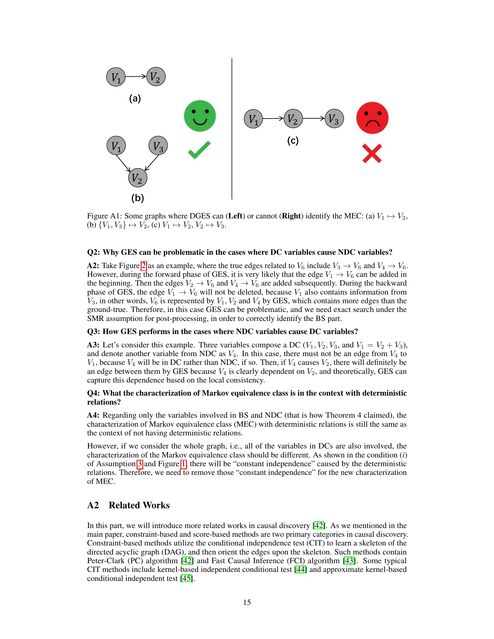
🔼 This figure shows three example graphs to illustrate the limitations of the DGES method in identifying the correct Markov equivalence class (MEC) when dealing with deterministic relations. Graph (a) and (b) can be correctly identified by DGES, while graph (c) cannot be identified because DGES would return a fully connected graph.
read the caption
Figure A1: Some graphs where DGES can (Left) or cannot (Right) identify the MEC: (a) V₁ → V₂, (b) {V₁, V₃} → V₂, (c) V₁ → V₂, V₂ ↔ V₃.

🔼 This figure presents the results of experiments conducted on simulated datasets with one minimal deterministic cluster. It compares the performance of different causal discovery methods (DPC, GES, A*, and DGES) across various settings (linear vs. non-linear models, varying numbers of variables and samples). The evaluation metrics used are Structural Hamming Distance (SHD), F1 score, precision, recall, and runtime.
read the caption
Figure 3: Results on the simulated datasets with one MinDC. We evaluate different functional causal models on varying number of variables and samples, respectively. For each setting, we consider SHD (↓), F₁ score (↑), precision (↑), recall (↑) and runtime (↓) as evaluation criteria.

In-depth insights
#

Deterministic Causality
#

Deterministic causality, where the cause directly and completely determines the effect without any probabilistic element, presents a unique challenge in causal inference. Traditional methods often rely on probabilistic assumptions, such as independent noise, which are violated in deterministic systems. This leads to difficulties in identifying causal relationships and accurately estimating causal effects. Score-based methods, particularly those using exact search, provide a more robust approach than constraint-based methods in handling deterministic settings. However, computational efficiency remains a significant hurdle, as exact search rapidly becomes intractable with increasing numbers of variables. The identifiability of causal structures under deterministic relations also requires careful consideration and relies on assumptions like sparsest Markov representation. Therefore, the development of efficient algorithms and a deeper understanding of identifiability conditions is crucial for advancing causal discovery in the presence of deterministic relationships.

DGES Framework
#

The Determinism-aware Greedy Equivalent Search (DGES) framework offers a novel approach to causal discovery by explicitly addressing the challenges posed by deterministic relationships in data. Its three-phase structure is key: first, identifying minimal deterministic clusters helps isolate subsets of variables with deterministic dependencies; second, a modified Greedy Equivalent Search (GES) algorithm, adapted to handle determinism, provides an initial causal graph; and third, precise exact search within these clusters and their neighbors refines the structure, leveraging the strengths of score-based methods while mitigating computational costs. DGES is designed for generality, accommodating both linear and nonlinear relationships, and handling continuous and discrete data types. Its theoretical grounding, particularly the identifiability conditions under mild assumptions, makes it a robust and significant contribution to causal inference. By combining the efficiency of GES with the accuracy of exact search, DGES provides a practical solution to a long-standing problem in causal discovery. The framework’s ability to detect and incorporate deterministic relations directly improves the accuracy and reliability of causal graph estimation.

Identifiability Limits
#

The concept of “Identifiability Limits” in causal discovery research is critical because it defines the inherent boundaries of what we can reliably infer from observational data. It highlights that even with perfect data and powerful algorithms, some causal relationships might remain ambiguous or unidentifiable. This is especially true in the presence of complex systems, latent confounders, or deterministic relationships, where traditional assumptions of causal inference models can be violated. Understanding identifiability limits helps researchers set realistic expectations about the scope and reliability of causal discovery, prompting them to carefully consider limitations and potential biases in their analyses. Furthermore, exploring these limits can drive methodological innovation, leading to the development of new algorithms or techniques to address these challenges and improve the accuracy and scope of causal inferences. A deep understanding of identifiability limits, therefore, is fundamental to responsible causal inference. By acknowledging these inherent limitations, researchers can focus on improving the design of studies, data collection methods, and analytical techniques to overcome these limitations and produce more robust and reliable results, advancing the field of causal inference significantly.

Empirical Validation
#

A robust empirical validation section is crucial for establishing the credibility of any research paper. It should present a comprehensive evaluation of the proposed method, comparing its performance against established baselines across a diverse range of datasets and scenarios. Clear descriptions of the datasets used, including their characteristics (size, dimensionality, noise levels, etc.), are essential. The choice of evaluation metrics should be justified and aligned with the research goals. The use of statistical significance tests should be highlighted, quantifying the extent to which observed performance differences are not due to chance. Visualizations such as graphs and tables should effectively communicate results, making it easier for the reader to understand patterns and trends. A thoughtful discussion of the findings, exploring potential limitations of the method and areas where further improvements are needed, contributes to the paper’s overall impact and strengthens its claim of significance. Finally, the reproducibility of the empirical validation is critical. Clear descriptions of experimental setup, including any hyperparameter settings, computing resources, and code availability, ensure that the findings can be verified independently.

Future Research
#

Future research directions stemming from this work on causal discovery with deterministic relations could explore several key areas. Extending the DGES framework to handle more complex scenarios such as those with latent confounders or selection bias is crucial. Improving the scalability of the exact search phase is another critical need, perhaps through the development of more efficient algorithms or heuristics. Investigating the impact of different score functions and their properties under deterministic settings warrants further investigation. Finally, applying the DGES methodology to real-world datasets in diverse domains and evaluating its performance in comparison to existing methods will validate its effectiveness and highlight its limitations. This could significantly advance the field’s practical applicability and provide valuable insights into the nuances of causal inference under deterministic conditions.

More visual insights
#

More on figures

🔼 This figure illustrates how the greedy equivalence search (GES) algorithm can produce incorrect results when dealing with deterministic relationships. In (a), the true causal graph is shown, with a deterministic cluster (DC) {V₁, V₂, V₃, V₄} and a non-deterministic cluster (NDC) {V₅, V₆, V₇}. The bridge set (BS) represents the edges connecting the DC and NDC. In (b), a possible DAG produced by GES is shown. GES incorrectly adds edges (BS’) resulting in a different structure than the true graph in (a). This highlights a limitation of GES when dealing with deterministic relationships that violate the faithfulness assumption.
read the caption
Figure 2: An example graph where V₁ = f(V₂, V₃, V₄). (a) the true graph where DC = {V₁, V₂, V₃, V₄}, NDC = {V₅, V₆, V₇}, and BS = {V₂→V₅, V₃→V₆, V₄→V₆}. (b) one possible DAG from the estimated CPDAG by GES, where BS' = {V₂→V₅, V₁→V₆, V₂→V₆, V₄→V₆}

🔼 This figure displays the results of experiments conducted on simulated datasets with one minimal deterministic cluster. The experiments compare the performance of different causal discovery methods (DPC, GES, A*, DGES) using linear and non-linear causal models. The metrics used to evaluate performance include Structural Hamming Distance (SHD), F1 score, precision, recall, and runtime. The results are shown across varying numbers of variables and samples.
read the caption
Figure 3: Results on the simulated datasets with one MinDC. We evaluate different functional causal models on varying number of variables and samples, respectively. For each setting, we consider SHD (↓), F₁ score (↑), precision (↑), recall (↑) and runtime (↓) as evaluation criteria.

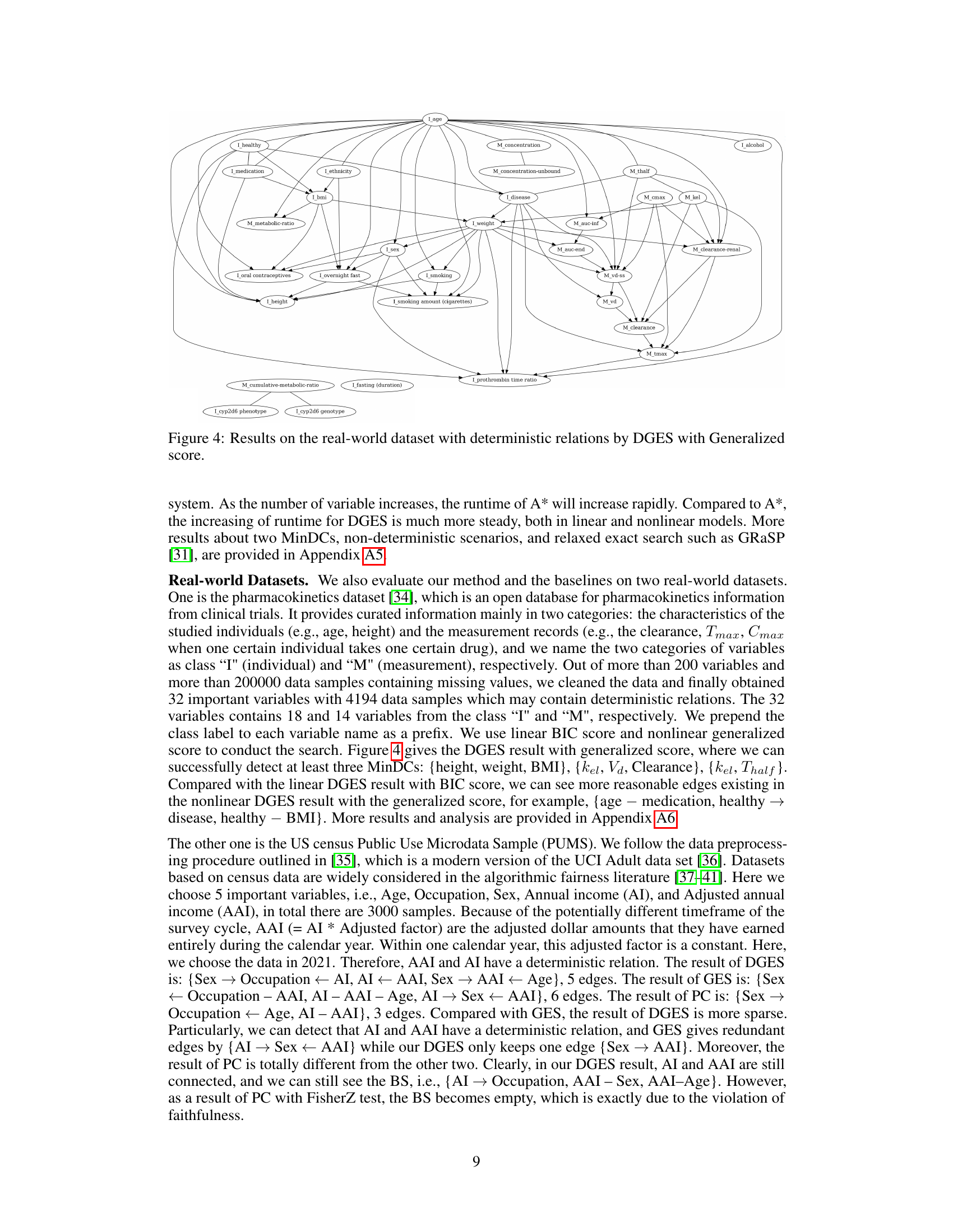
🔼 This figure displays the causal graph learned by the Determinism-aware Greedy Equivalent Search (DGES) method using the generalized score on a real-world pharmacokinetics dataset. The graph shows the relationships between various individual characteristics (e.g., age, sex, ethnicity, medication use) and pharmacokinetic measurements (e.g., drug concentration, clearance, volume of distribution). The DGES method specifically identifies and handles deterministic relations within the data, leading to a potentially more accurate representation of the causal structure compared to methods that don’t account for determinism.
read the caption
Figure 4: Results on the real-world dataset with deterministic relations by DGES with Generalized score.

🔼 This figure shows three example graphs illustrating scenarios where the Determinism-aware Greedy Equivalent Search (DGES) method can or cannot correctly identify the Markov equivalence class (MEC). In graphs (a) and (b), DGES successfully identifies the MEC. However, in graph (c), DGES fails to correctly identify the MEC due to the complexities introduced by the deterministic relationships.
read the caption
Figure A1: Some graphs where DGES can (Left) or cannot (Right) identify the MEC: (a) V₁ → V₂, (b) {V₁, V₃} → V₂, (c) V₁ → V₂, V₂ V₃.

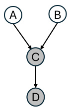
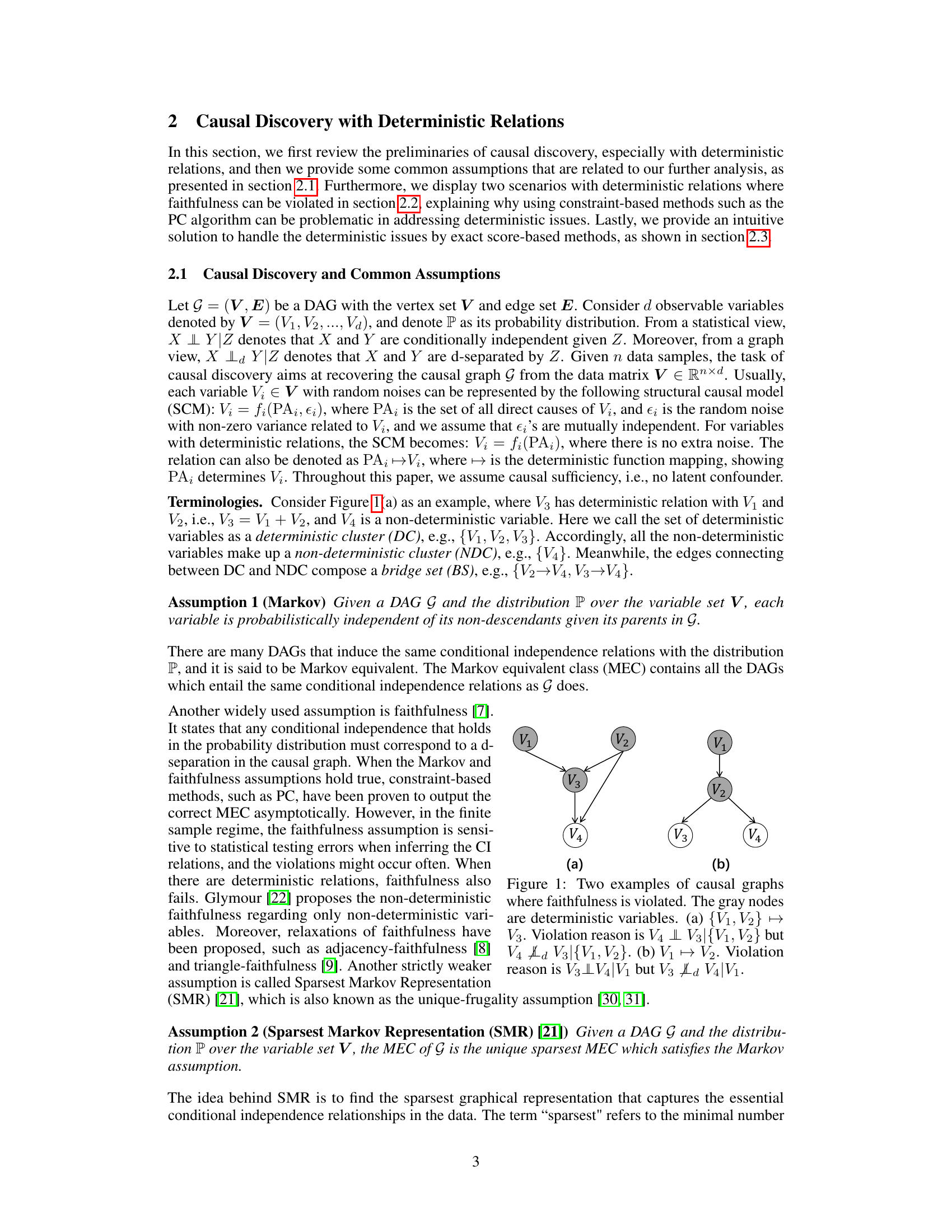
🔼 This figure shows two examples of causal graphs where the faithfulness assumption is violated due to deterministic relationships. In (a), the deterministic relationship between V1, V2, and V3 causes a conditional independence between V3 and V4 given V1 and V2, which violates faithfulness. In (b), a similar violation occurs due to a deterministic relationship between V1 and V2 and a conditional independence between V3 and V4 given V1.
read the caption
Figure 1: Two examples of causal graphs where faithfulness is violated. The gray nodes are deterministic variables. (a) {V1, V2} → V3. Violation reason is V4 ⊥ V3|{V1, V2} but V4 ⫫ V3|{V1, V2}. (b) V1 → V2. Violation reason is V3⊥V4|V1 but V3 ⫫ V4|V1.

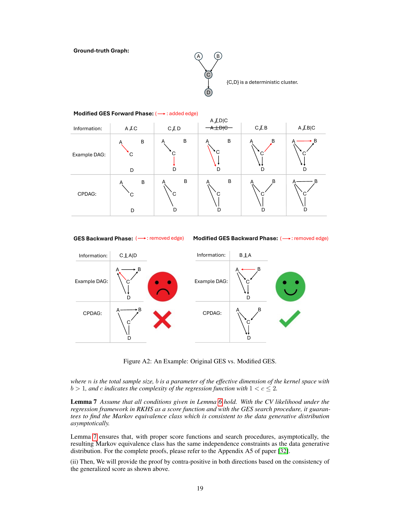
🔼 This figure demonstrates the difference between the original GES algorithm and the modified GES algorithm proposed in the paper. The original GES algorithm, when applied to a graph containing deterministic relations, can incorrectly add or remove edges due to spurious conditional independencies caused by determinism. This example shows how the modified GES algorithm addresses this issue by incorporating additional constraints in the forward and backward phases of the search, ensuring that the resulting graph accurately reflects the causal relationships even in the presence of deterministic clusters. The modified GES algorithm improves the accuracy of the causal graph estimation by handling deterministic relations more effectively.
read the caption
Figure A2: An Example: Original GES vs. Modified GES.

🔼 This figure shows three example graphs to illustrate the limitations of the DGES method in identifying causal relationships involving deterministic clusters. The graphs demonstrate scenarios where DGES can successfully identify the true Markov equivalence class (MEC) and scenarios where it fails. The key factor appears to be the structure of connections between deterministic (shaded nodes) and non-deterministic nodes. The analysis highlights that the method cannot always accurately determine the causal skeleton and directions within the deterministic clusters (MinDCs) when the deterministic relations are complex or involve overlapping variables.
read the caption
Figure A1: Some graphs where DGES can (Left) or cannot (Right) identify the MEC: (a) V₁ → V₂, (b) {V₁, V₃} → V₂, (c) V₁ → V₂, V₂ V₃.

🔼 This figure presents the results of experiments on simulated datasets with one minimal deterministic cluster (MinDC). The experiments evaluate the performance of different causal discovery methods under various settings, including linear Gaussian models, general nonlinear models, and varying numbers of variables and samples. The evaluation metrics used are Structural Hamming Distance (SHD), F1 score, precision, recall, and runtime, with lower SHD and higher values for F1 score, precision, and recall indicating better performance. The figure displays these metrics across different models and dataset sizes, allowing a comparison of their effectiveness under various conditions.
read the caption
Figure 3: Results on the simulated datasets with one MinDC. We evaluate different functional causal models on varying number of variables and samples, respectively. For each setting, we consider SHD (↓), F₁ score (↑), precision (↑), recall (↑) and runtime (↓) as evaluation criteria.

🔼 This figure presents the results of experiments conducted on simulated datasets containing a single minimal deterministic cluster (MinDC). Five different metrics were used to evaluate the performance of the proposed method (DGES) against three baseline methods (DPC, GES, A*): Structural Hamming Distance (SHD), F1 score, precision, recall, and runtime. Experiments were performed across various numbers of variables and samples to assess the efficacy of DGES under linear and nonlinear causal relationships. The arrow notation (↓) indicates lower is better and (↑) indicates higher is better for each metric.
read the caption
Figure 3: Results on the simulated datasets with one MinDC. We evaluate different functional causal models on varying number of variables and samples, respectively. For each setting, we consider SHD (↓), F₁ score (↑), precision (↑), recall (↑) and runtime (↓) as evaluation criteria.

🔼 The figure shows the performance comparison of different causal discovery methods (DPC, GES, A*, DGES, GRaSP) on simulated datasets with one minimal deterministic cluster (MinDC). The experiments vary the number of variables and samples, using linear Gaussian and nonlinear models with mixed functions. The results are evaluated using structural Hamming distance (SHD), F1 score, precision, recall, and runtime. Lower SHD and higher F1 score, precision, and recall are better, while lower runtime is preferred.
read the caption
Figure 3: Results on the simulated datasets with one MinDC. We evaluate different functional causal models on varying number of variables and samples, respectively. For each setting, we consider SHD (↓), F₁ score (↑), precision (↑), recall (↑) and runtime (↓) as evaluation criteria.

🔼 This figure shows the results of applying the Determinism-aware Greedy Equivalent Search (DGES) method with a generalized score to a real-world dataset containing deterministic relations. The graph visually represents the causal relationships discovered by the algorithm among various variables. The nodes represent variables, and the edges represent the causal relationships between them. The figure is used to demonstrate the efficacy of the DGES method in handling real-world data.
read the caption
Figure 4: Results on the real-world dataset with deterministic relations by DGES with Generalized score.

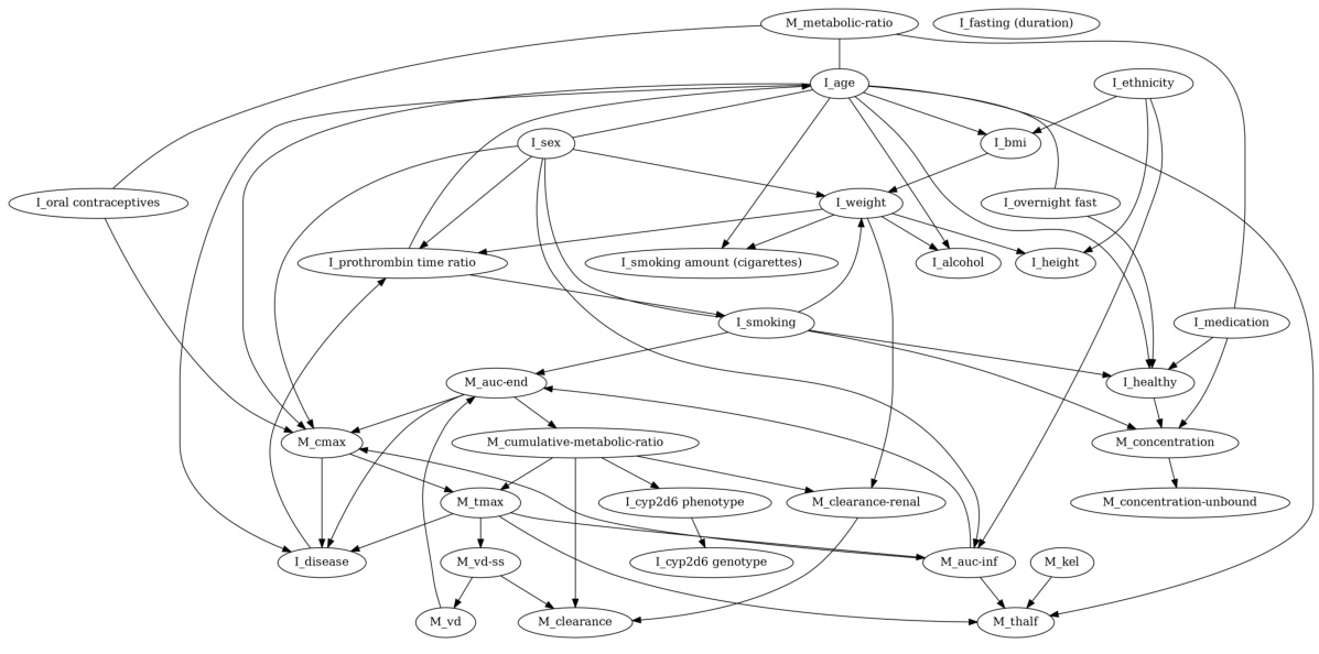
🔼 This figure shows the causal graph learned by the Determinism-aware Greedy Equivalent Search (DGES) method on a real-world pharmacokinetics dataset. The graph includes both deterministic and non-deterministic relationships. The nodes represent variables (individual characteristics and measurement results), and the edges represent causal relationships inferred by the algorithm. The use of a generalized score function allows DGES to handle both linear and non-linear relationships.
read the caption
Figure 4: Results on the real-world dataset with deterministic relations by DGES with Generalized score.

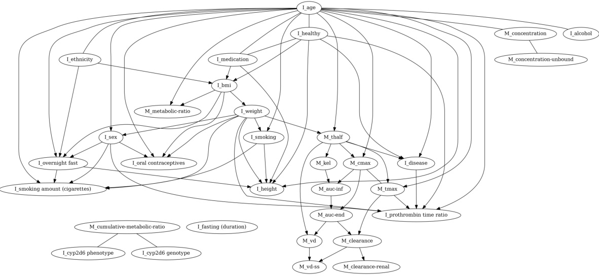
🔼 This figure shows the causal graph learned by the Determinism-aware Greedy Equivalent Search (DGES) method on a real-world pharmacokinetics dataset. The graph visually represents the causal relationships between different variables in the dataset, particularly highlighting the relationships involving deterministic variables like BMI (body mass index), which is calculated from weight and height. The use of a generalized score in DGES allows the method to handle both linear and nonlinear causal relationships, providing a comprehensive view of the causal structure in the presence of deterministic relations. The edges in this graph indicate the causal links identified by DGES; their absence indicates a lack of causal relationship.
read the caption
Figure 4: Results on the real-world dataset with deterministic relations by DGES with Generalized score.

TL;DR#

Key Takeaways#

Why does it matter?#

Visual Insights#

In-depth insights#

Deterministic Causality#

DGES Framework#

Identifiability Limits#

Empirical Validation#

Future Research#

More visual insights#

Full paper#