↗ OpenReview ↗ NeurIPS Homepage ↗ Chat
TL;DR#
Transfer learning in network analysis is challenging due to limited data and complex relationships between networks. Existing methods often struggle to handle these challenges effectively, leading to suboptimal estimation of target networks. This research addresses this problem by focusing on latent variable network models, leveraging information from related source networks to enhance the estimation of target networks.
The proposed approach utilizes a novel algorithm that leverages the ordering of a suitably defined graph distance. This algorithm achieves vanishing error under specific conditions and does not rely on restrictive assumptions about the network structures. Furthermore, this paper provides a minimax lower bound and demonstrates that a simpler algorithm attains this rate in the specific case of stochastic block models. The effectiveness of the proposed method is demonstrated using simulations and real-world datasets, showing significant performance gains over existing methods.
Key Takeaways#
Why does it matter?#
This paper is important because it addresses the critical challenge of transfer learning in network analysis, a rapidly growing field with numerous applications. The proposed efficient algorithms and theoretical results provide valuable tools and insights for researchers, advancing the understanding and application of transfer learning in complex network settings. This work opens new avenues for research in various domains, such as biological network analysis, social network analysis, and recommendation systems, where effectively leveraging limited data from related sources is crucial.
Visual Insights#

This figure compares the performance of three algorithms (Algorithm 1, Algorithm 2, and Oracle with p=0.1) on three different source-target pairs of networks. Each row represents a different pair, with the true source network (P) shown in the upper left triangle of the first column. The heatmaps compare the true target matrix (Q) (lower left triangle) to the estimated target matrices produced by the three algorithms (upper right triangle). The figure demonstrates that Algorithm 2 is most accurate when both the source and target networks are stochastic block models (SBMs), while Algorithm 1 performs better for smooth graphons.

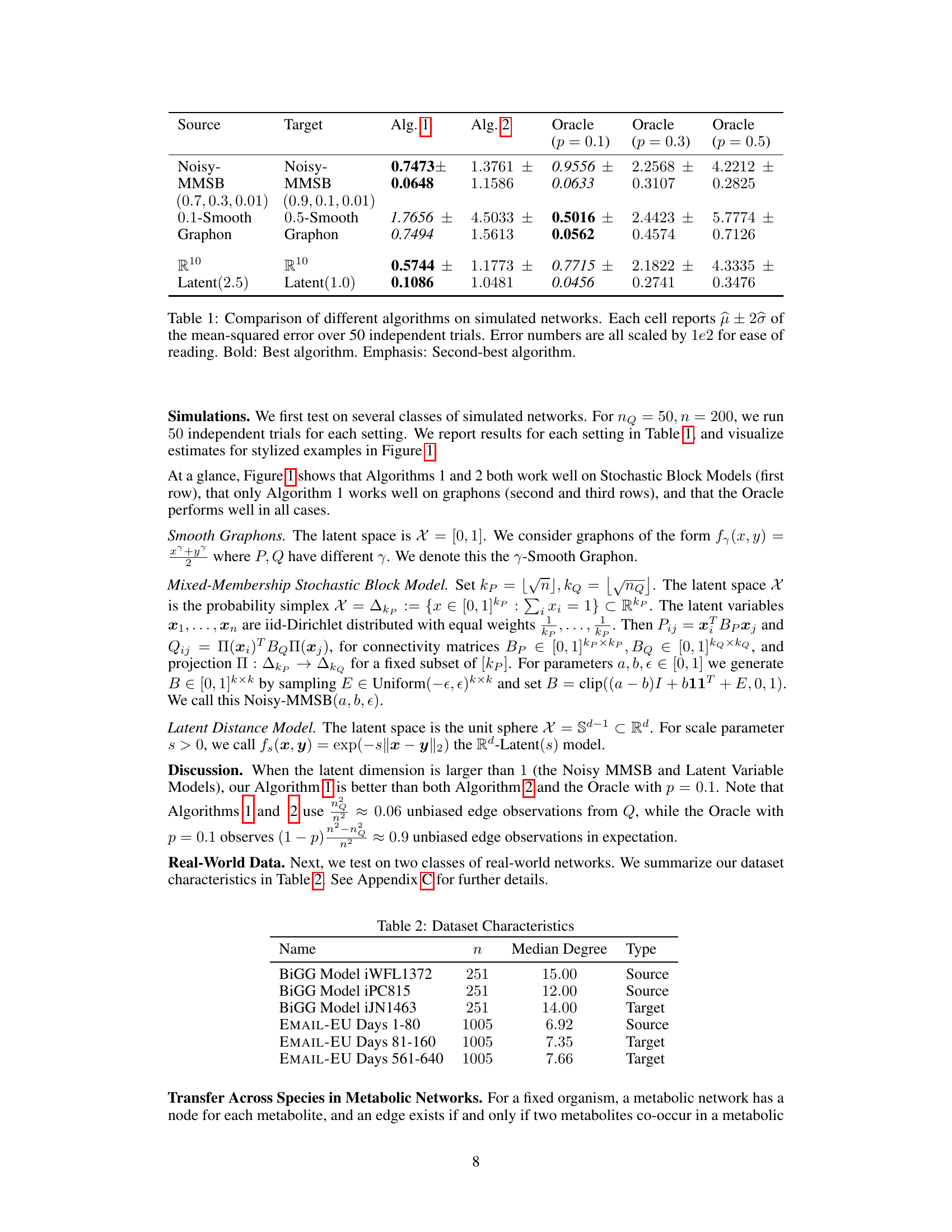
The table compares the performance of three algorithms (Algorithm 1, Algorithm 2, and Oracle) on six simulated network datasets. The algorithms are evaluated based on their mean squared error (MSE), with error bars representing ±2 standard deviations. The MSE values are scaled by a factor of 100. The ‘Oracle’ represents an ideal scenario with full access to data, while Algorithms 1 and 2 leverage transfer learning. The best performing algorithm for each dataset is highlighted in bold, with the second-best in italics.
In-depth insights#
Network Transfer#
Network transfer learning, a crucial aspect of machine learning, focuses on leveraging knowledge gained from a source network to enhance the learning process on a target network. This is particularly useful when labeled data for the target network is scarce or expensive to obtain. The core challenge lies in effectively transferring relevant information across networks, especially when they exhibit structural differences. Successful transfer relies on identifying shared latent structures or features between the source and target networks, allowing for knowledge generalization. Algorithms often exploit shared latent variables, graph distances, or community structures to facilitate knowledge transfer. However, the presence of edge correlations in network data introduces unique complexities. Evaluating the effectiveness of network transfer demands careful consideration of factors such as network structure, data volume, and the similarity between source and target domains. The choice of transfer learning algorithm significantly influences performance. Future research needs to address challenges like handling differing network structures and developing robust performance metrics tailored specifically for network transfer.
Latent Variable Models#
The section on ‘Latent Variable Models’ would ideally delve into the theoretical underpinnings of these models, highlighting their suitability for network analysis. It should emphasize that these models posit the existence of latent variables influencing observed network connections, moving beyond simple random graph assumptions. Stochastic Block Models (SBMs) and random dot product graphs are key examples that should be mentioned, along with a discussion of their strengths and limitations. A crucial aspect would be explaining how the latent variables (often representing community memberships or node features) shape edge probabilities, resulting in the observed network structure. The discussion should touch upon the challenges of estimating these models, particularly when dealing with partially observed or noisy data. Finally, the relevance to the paper’s transfer learning methodology should be clearly articulated, emphasizing how the shared latent structure across source and target networks enables knowledge transfer, potentially offering a more nuanced understanding of network relationships than traditional methods.
Algorithm Analysis#
An Algorithm Analysis section in a research paper would ideally delve into the time and space complexity of proposed algorithms, using Big O notation to express their scalability. A rigorous analysis would consider best, average, and worst-case scenarios, providing a comprehensive picture of performance under varying conditions. Proofs of correctness, or at least strong arguments for correctness, should be included to verify the algorithm’s functionality. The analysis should extend beyond simple complexity measures to include discussions of algorithm efficiency compared to existing methods, ideally supported by both theoretical comparisons and experimental results. Crucially, the analysis should highlight any limitations of the proposed approach, such as reliance on specific data characteristics or computational bottlenecks. Empirical evaluation is often also included in this section, which might involve executing algorithms on various datasets and reporting on resource usage (CPU time, memory) and solution quality. Ideally, a discussion of trade-offs between different algorithms, perhaps using a table summarizing their performance characteristics, helps the reader understand the choices made in algorithm design.
Minimax Lower Bounds#
Minimax lower bounds represent a fundamental concept in statistical decision theory, offering a benchmark for the best achievable performance of any estimator. They establish a lower limit on the expected error, regardless of the specific estimation method employed. In the context of a research paper, a section on minimax lower bounds would likely detail the derivation of such a bound, often using techniques like Assouad’s Lemma or Fano’s inequality. These derivations would typically involve constructing a challenging set of hypotheses (e.g., different network structures or model parameters) to prove the impossibility of achieving error rates below a certain level. The significance lies in providing a rigorous theoretical foundation, demonstrating that certain levels of estimation error are unavoidable given limited data. The results can then be used to compare the performance of proposed estimators against this inherent limitation, helping to evaluate their efficiency and optimality. The strength of a minimax lower bound analysis depends on how tightly the bound reflects the true difficulty of the problem; a loose bound might not effectively inform the evaluation of estimators.
Real-World Networks#
The application of transfer learning methodologies to real-world networks, particularly focusing on metabolic and email networks, is a crucial aspect of this research. The study demonstrates the effectiveness of the proposed algorithms in these diverse settings. Metabolic networks, with their intricate structures and limited observational data, pose a significant challenge. The findings highlight how transfer learning, by leveraging data from related source networks, can improve the accuracy of estimations for target metabolic networks where complete data is scarce. Similarly, the analysis of email communication networks showcases the algorithm’s adaptability and performance. This real-world application reinforces the potential of transfer learning as a powerful tool for analyzing complex networks with limited data and diverse characteristics. However, further investigation is needed to address challenges such as the choice of appropriate source networks and the robustness of algorithms in scenarios with significant structural differences between source and target networks. This would solidify the practical applicability of transfer learning across varied real-world network types.
More visual insights#
More on figures

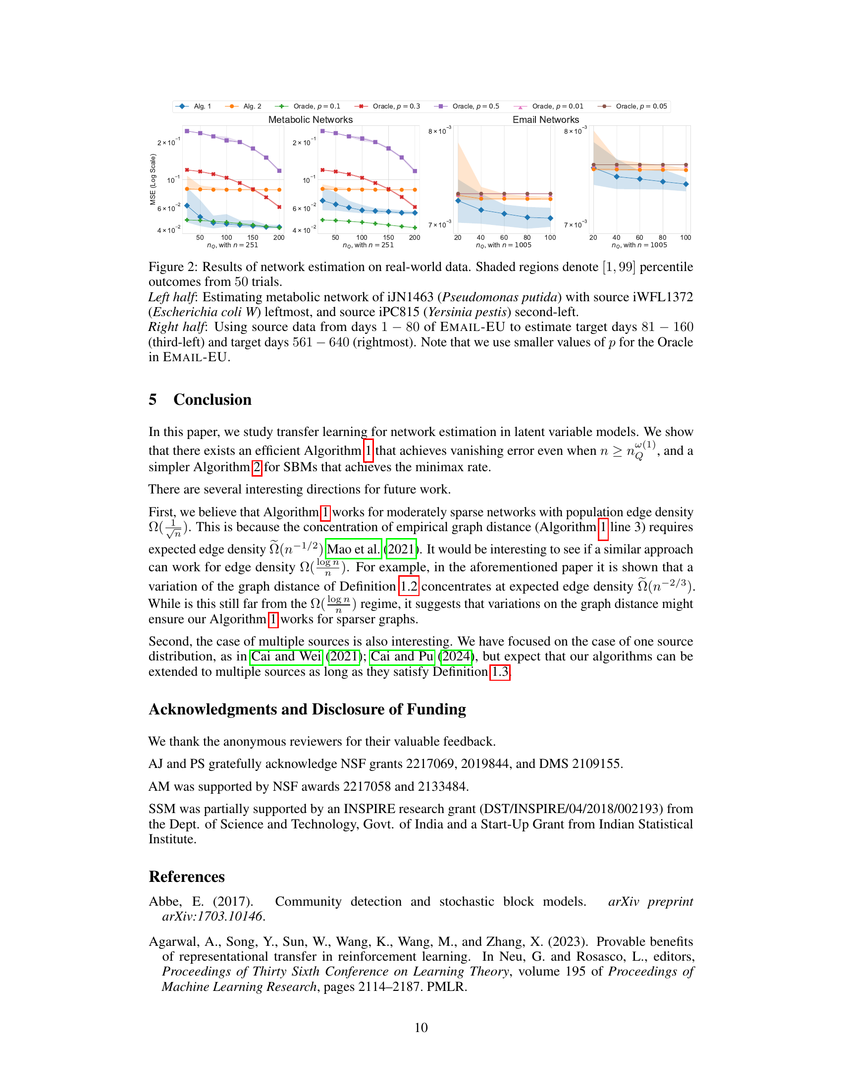
This figure compares the performance of the proposed algorithms (Algorithm 1 and Algorithm 2) and the oracle method on real-world datasets. The left half shows the results for metabolic networks, where the target network is the metabolic network of Pseudomonas putida, and the source networks are the metabolic networks of Escherichia coli and Yersinia pestis. The right half shows the results for email networks, where the target networks are the email interaction networks from different time periods, and the source network is the email interaction network from an earlier period. The shaded regions show the 98% confidence intervals for the mean-squared error (MSE) of the different methods.
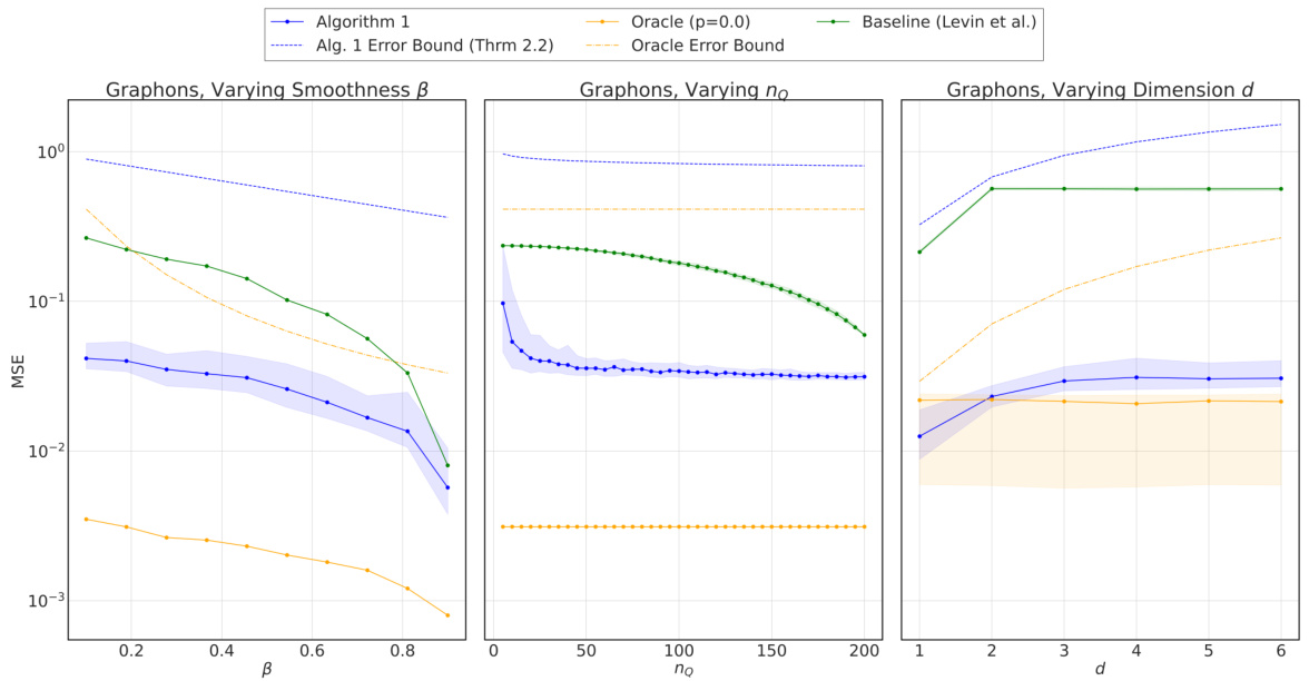
This figure presents the results of testing Algorithm 1’s performance under varying parameters for latent variable models. The left panel shows the impact of smoothness (β) on the mean squared error (MSE). The middle panel illustrates the effect of the number of observed target nodes (nQ) on the MSE. The right panel examines the influence of latent space dimensionality (d) on the MSE. For most parameter settings, Algorithm 1 outperforms the baseline but underperforms the oracle, demonstrating its effectiveness in transfer learning.

This figure displays the results of testing Algorithm 2’s performance on Stochastic Block Models (SBMs). The left panel shows how the mean squared error (MSE) changes with varying numbers of observed target nodes (nq), while the right panel shows the impact of varying the number of communities (kq) in the target model. In both cases, the performance of Algorithm 2 is compared to an oracle and a baseline method. The shaded areas represent the 5th to 95th percentile range of MSE across 50 trials, demonstrating the variability of the results.
This figure compares the performance of three algorithms (Algorithm 1, Algorithm 2, and Oracle) on three different source-target pairs of networks. Each row represents a different pair, and the heatmaps show the estimated probability matrices (Q) produced by each algorithm compared to the true probability matrices (P and Q). The results show that Algorithm 2 is most effective for Stochastic Block Models, while Algorithm 1 performs better for smooth graphons. The Oracle method, which has access to complete target data, performs well in all cases.
The figure compares three algorithms (Algorithm 1, Algorithm 2, and Oracle) for estimating the target network Q using transfer learning from a source network P. It shows heatmaps representing the estimated and true probability matrices for three different source-target pairs. Algorithm 2 performs best on stochastic block models, whereas Algorithm 1 is superior for smooth graphons. The Oracle algorithm serves as a performance benchmark.
This figure compares the performance of three algorithms (Algorithm 1, Algorithm 2, and Oracle) on three different source-target network pairs with varying network structures (Stochastic Block Model, Smooth Graphons). It visually demonstrates the accuracy of each algorithm in reconstructing the target network (Q) using limited target data and complete source data (P). The heatmaps represent the adjacency matrices of the true networks and the estimated networks, illustrating the differences between them.
This figure compares the performance of three different algorithms (Algorithm 1, Algorithm 2, and Oracle) in estimating the target network Q from the source network P and limited target data. It presents the results for three different pairs of source and target networks which have different characteristics (Stochastic Block Models, smooth graphons). Each heatmap visualization shows the true P and Q for each network pair and the estimated Q for the three algorithms. The results suggest that Algorithm 2 is superior when the networks are Stochastic Block Models, while Algorithm 1 performs better for smooth graphons.
Full paper#
