↗ OpenReview ↗ NeurIPS Homepage ↗ Chat
TL;DR#
Many real-world applications utilize tabular data, but existing neural network architectures lack inherent explainability. This poses challenges when decisions based on model predictions need to be transparent and justifiable, particularly in sensitive domains like healthcare or finance. The need for high-performing yet explainable models is a crucial open research question.
This research introduces Interpretable Mesomorphic Neural Networks (IMNs). IMNs leverage deep hypernetworks to generate explainable linear models on a per-instance basis. This approach allows IMNs to maintain the accuracy of deep networks while offering explainability by design. Extensive experiments show that IMNs achieve performance on par with state-of-the-art black-box models, while significantly outperforming existing explainable methods. The local linearity of the models makes it easy to interpret predictions, thereby boosting the trust and transparency of AI systems.
Key Takeaways#
Why does it matter?#
This paper is important because it introduces a novel class of interpretable neural networks for tabular data, addressing the critical need for explainable AI in real-world applications. It offers a new design paradigm, achieving comparable accuracy to black-box models while providing free-lunch explainability. This opens avenues for future research in explainable deep learning and the development of more trustworthy AI systems, particularly in domains demanding transparency and accountability.
Visual Insights#

The figure illustrates the architecture of the Interpretable Mesomorphic Network (IMN). It shows a TabResNet backbone that feeds into a ResNet MLP with parameters θ. This MLP acts as a hypernetwork, generating the interpretable linear model weights w(x;θ) for a given input data point x. The weights w(x; θ) are then used to generate the prediction ŷ as a linear combination with the input x: ŷ = xTw(x; θ). The figure visually distinguishes the different layers of the network using different colors and shapes for the nodes. The IMN architecture combines the accuracy of deep networks with the interpretability of linear models.
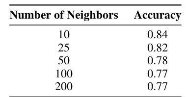
This table shows the accuracy of the local hyperplanes generated by the IMN model for different numbers of neighboring points. The accuracy is calculated by using the hyperplane generated for a single data point to classify its neighbors. The table demonstrates that the IMN model generates hyperplanes that maintain reasonable accuracy even when classifying points further away from the data point for which the hyperplane was originally trained.
In-depth insights#
IMN Architecture#
The IMN architecture is a novel approach that leverages deep hypernetworks to generate instance-specific linear models for tabular data. This design cleverly combines the advantages of deep learning’s ability to capture complex relationships with the interpretability of linear models. The hypernetwork acts as a feature selector, identifying relevant features for each data point, generating a linear model tailored to that specific instance. Local linear models provide explainability by design, while the deep hypernetwork ensures that the model can still achieve high accuracy. The architecture is not just about combining two model types; it’s a synergistic design where the hypernetwork learns to generate linear models that are both accurate and interpretable. This approach offers an elegant solution to the long-standing challenge of reconciling accuracy and explainability in deep learning for tabular data. End-to-end training further enhances the model’s effectiveness and facilitates seamless integration of interpretability.**
Explainability via IMN#
The core idea of “Explainability via IMN” revolves around using interpretable mesomorphic neural networks (IMNs) to enhance the transparency of deep learning models applied to tabular data. IMNs cleverly combine the accuracy of deep networks with the inherent interpretability of linear models. This is achieved by training deep hypernetworks that generate instance-specific linear models. These linear models offer straightforward explanations, unlike the “black box” nature of many deep learning models. The process is end-to-end, meaning that the hypernetwork learns to directly produce accurate and readily interpretable linear models that also classify or predict well, thereby providing a built-in mechanism for explaining individual predictions. A key advantage is the comparable accuracy to black-box models, while maintaining easy-to-understand explanations, a significant advancement in explainable AI. This approach addresses the challenge of balancing predictive performance with model transparency, especially in the context of tabular datasets often used in critical decision-making domains. The IMN framework offers a potential solution to the explainability problem in deep learning, enhancing trust and accountability for the predictions generated.
Accuracy & IMN#
The accuracy of Interpretable Mesomorphic Networks (IMNs) is a central theme. The paper demonstrates that IMNs achieve comparable accuracy to state-of-the-art black-box models on various tabular datasets, a significant finding given their design for interpretability. This suggests that the inclusion of interpretability does not necessarily compromise predictive performance. Furthermore, IMNs often outperform existing explainable-by-design models, highlighting their advantage in balancing accuracy and explainability. The consistency of IMN’s accuracy across different datasets and experimental conditions strengthens the results, indicating robustness and generalizability. Global accuracy and local interpretability are shown to coexist effectively, indicating that local linear models generated by the IMNs effectively capture the decision boundary’s complexity. The study uses extensive empirical evaluation on multiple benchmarks to solidify its claims regarding accuracy, emphasizing the practical relevance of IMNs for real-world applications.
IMN Interpretability#
The IMN (Interpretable Mesomorphic Network) approach centers on generating locally linear models via deep hypernetworks. This design enables inherent interpretability because the resulting linear models directly reveal feature importance through their weights. The weights themselves, produced by a deep hypernetwork, are not directly interpretable; however, their output – the linear model parameters – are. This per-instance linearity allows for straightforward attribution of feature influence on a prediction’s magnitude and sign. While global interpretability isn’t directly built into the hypernetwork, the aggregation of these local linear model weights across the dataset provides a measure of global feature importance. The tradeoff is that local linearity might sacrifice some predictive accuracy compared to a complex, black-box model. However, the results show comparable performance to black-box methods with state-of-the-art explainability.
Future of IMN#
The future of Interpretable Mesomorphic Networks (IMN) looks promising, particularly in addressing the limitations of current explainable AI models. IMN’s unique mesomorphic architecture, combining depth for accuracy with linearity for interpretability, could be significantly enhanced. Future research could explore non-linear interpretable models generated by the hypernetwork, expanding beyond simple linear models to capture complex interactions in data. Additionally, scalability is crucial. While IMN demonstrates promising results, investigating its performance on extremely large datasets and high-dimensional features will be vital to its widespread adoption. Finally, expanding IMN’s application beyond tabular data and into other modalities, such as images and text, using suitable backbone networks, offers exciting possibilities for broader impact. This would require careful consideration of how the hypernetwork generates explainable representations within the chosen modality. Integrating IMN with other XAI techniques to offer a multi-faceted approach to model explanation is another promising avenue. Overall, a focused effort on these aspects—model complexity, scalability, and generalizability—will significantly contribute to IMN’s maturation and influence in the field of XAI.
More visual insights#
More on figures

The figure demonstrates the accuracy and interpretability of the proposed Interpretable Mesomorphic Networks (IMN). The left panel shows the global decision boundary learned by IMN, illustrating its ability to accurately separate classes in a non-linear fashion. The right panel highlights the local interpretability aspect, showing a local hyperplane generated for a single data point (x’). This hyperplane not only correctly classifies x’ but also generalizes well to its neighboring points, indicating that IMN generates accurate local linear models that offer good global classification performance.

This figure shows the results of comparing several white-box interpretable methods (Decision Tree, Logistic Regression, and IMN) using the average rank across multiple datasets. A lower average rank indicates superior performance. The critical difference (CD) is shown to demonstrate statistically significant differences in performance between methods.

The figure demonstrates the accuracy and interpretability of the proposed Interpretable Mesomorphic Networks (IMN). The left panel shows the globally accurate non-linear decision boundary learned by IMN. The right panel illustrates the local interpretability by showing a local hyperplane generated for a single data point (x’). This hyperplane not only correctly classifies x’ but also generalizes well to its neighboring points, highlighting the model’s ability to provide both global accuracy and local interpretability simultaneously.

This figure displays the performance of various interpretability methods (IMN, SHAP, Kernel SHAP, LIME, Maple, L2X, BreakDown, Random, and TabNet) across four different metrics (Faithfulness (ROAR), Monotonicity (ROAR), Faithfulness, and Infidelity) on a Gaussian Linear dataset. The x-axis represents the degree of feature correlation (p), ranging from 0 to 1. The y-axis shows the metric values for each method. The figure helps to understand how each method’s interpretability changes based on the level of feature correlation in the dataset.

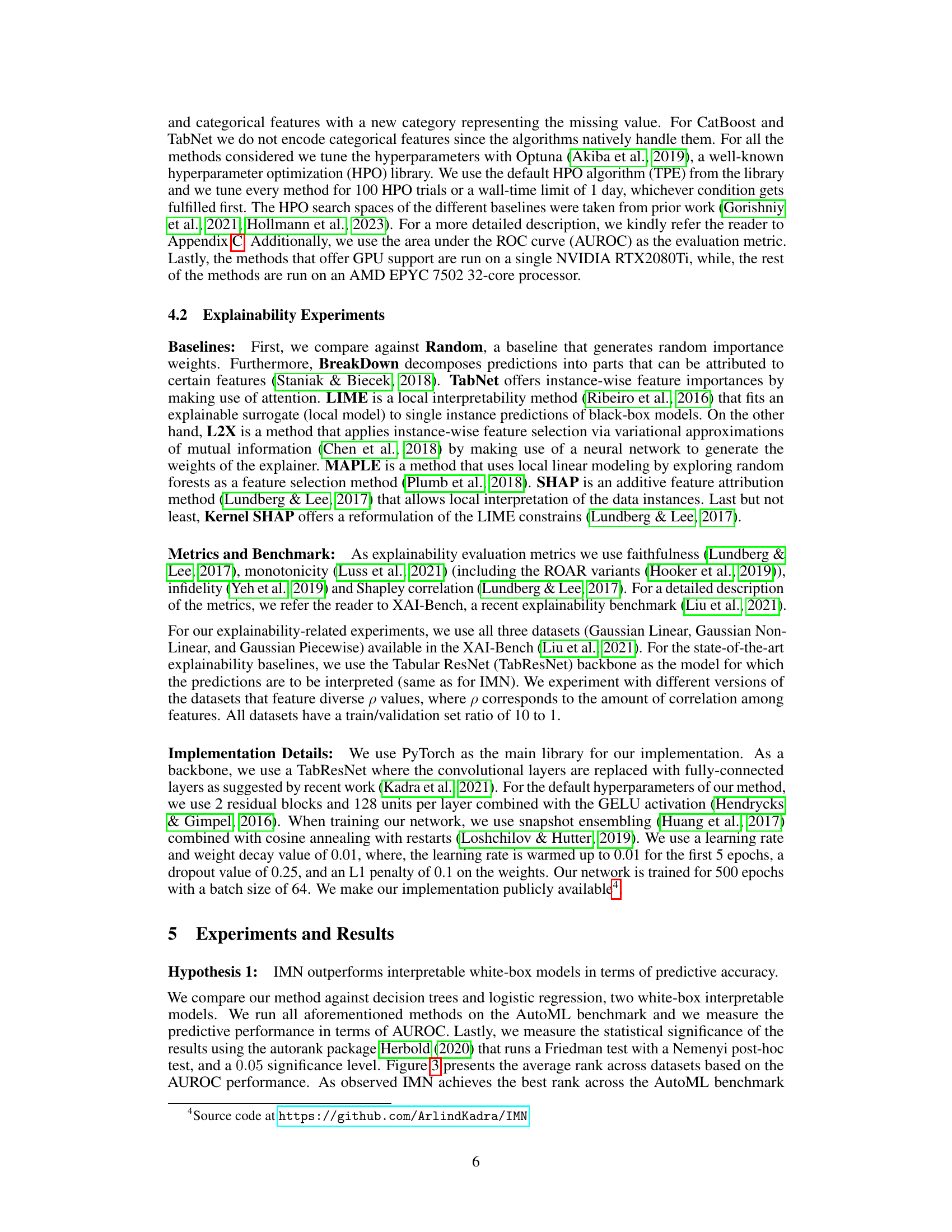
The figure shows a bar chart comparing the performance drop (in AUROC) of different models when removing the top-k most important features, as determined by each model’s feature attribution method. The x-axis represents the number of features removed (k). The y-axis represents the percentage decrease in AUROC. The chart helps to assess the relative importance of features identified by each model by observing how much performance is affected when those features are removed.
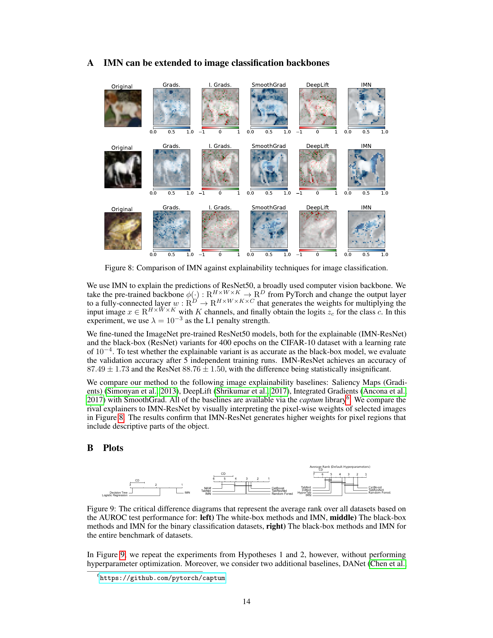
This figure compares the image classification results and visualizations of the proposed IMN method against several existing explainability techniques, including Gradient, Integrated Gradient, SmoothGrad, and DeepLift. The results demonstrate that IMN generates higher weights for regions of the image that are most descriptive of the object.

This figure compares the performance of IMN against other explainability techniques for image classification using the ResNet50 backbone. It shows visualizations of feature attribution maps generated by various methods (Gradients, Integrated Gradients, SmoothGrad, DeepLift, and IMN) for three different images. The color intensity in each map represents the importance assigned to each pixel in the prediction. This experiment demonstrates IMN’s ability to identify relevant image regions for prediction in a manner comparable to other existing methods.

This figure shows two plots that illustrate the global accuracy and local interpretability of the Interpretable Mesomorphic Networks (IMN) model. The left plot displays the global decision boundary learned by IMN, demonstrating its ability to accurately separate different classes in the dataset. The right plot focuses on a specific data point (x’) and shows that IMN generates a local hyperplane (a linear decision boundary) that correctly classifies not only x’, but also its neighboring data points. This highlights IMN’s capability to achieve both global accuracy and local interpretability simultaneously.

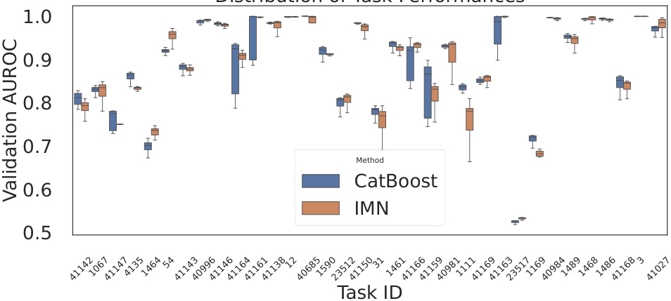
This figure shows the distribution of the performance gain of different machine learning models compared to a decision tree. The gain is calculated as the difference between the AUROC score of a model and the AUROC score of a decision tree, divided by the AUROC score of the decision tree. The box plot shows the median, quartiles, and outliers for each model. The figure demonstrates that most models show similar gains, but NAM (Neural Additive Model) performs considerably worse than the other models.

This figure displays the results of the interpretability experiment. The experiment compares IMN against other interpretability methods in the presence of feature correlations in the Gaussian Linear Dataset. The plot shows the performance of all methods on four metrics: faithfulness (ROAR), monotonicity (ROAR), faithfulness and infidelity. The performance is evaluated for different values of feature correlation, ranging from 0 to 1.
This figure compares the performance of different classification models using the AUROC metric. It shows critical difference diagrams, which visually represent the statistical significance of differences in average rank between various models. The diagrams are presented separately for white-box models, black-box models on binary classification datasets, and black-box models across all datasets in the benchmark. This allows a comparison of the relative performance and statistical significance of IMN against other interpretable and non-interpretable models in different experimental settings.
More on tables

This table presents the median training and inference times for various machine learning models used in the paper’s experiments. The models are categorized as either interpretable white-box models, strong black-box classifiers, or interpretable deep learning architectures. Training times reflect the time taken to train the models, while inference times reflect the time taken to generate predictions for a single data instance. The GPU usage for some of the models is also specified. This table provides a comparative analysis of the computational efficiency of different methods for both training and inference.
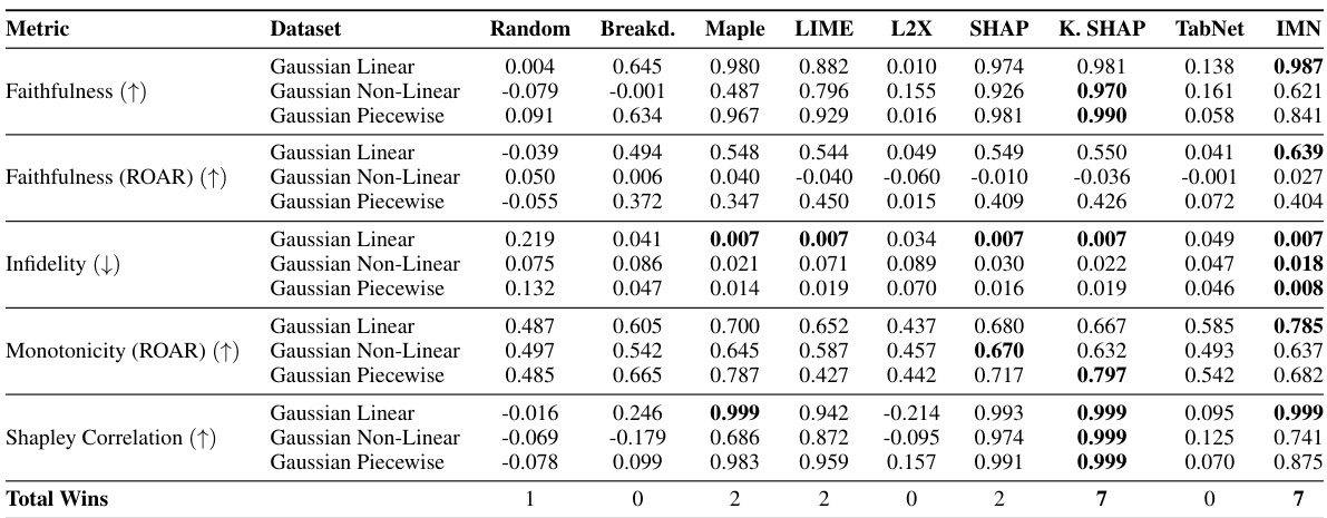
This table presents a comparison of the proposed IMN method against eight state-of-the-art explainability methods across three datasets from the XAI Benchmark. The comparison uses five interpretability metrics: Faithfulness, Faithfulness (ROAR), Infidelity, Monotonicity (ROAR), and Shapley Correlation. Higher values are better for Faithfulness and Monotonicity, while lower values are better for Infidelity. The table shows the performance of each method on each metric for each dataset, allowing for a comprehensive evaluation of the IMN’s interpretability compared to existing techniques.

This table presents the median inference time in seconds for various interpretable methods including IMN, TabNet, and SHAP using different backbones (TabResNet and CatBoost) on three benchmark datasets: Credit-g, Adult, and Christine. The results demonstrate IMN’s significantly faster inference compared to other methods.

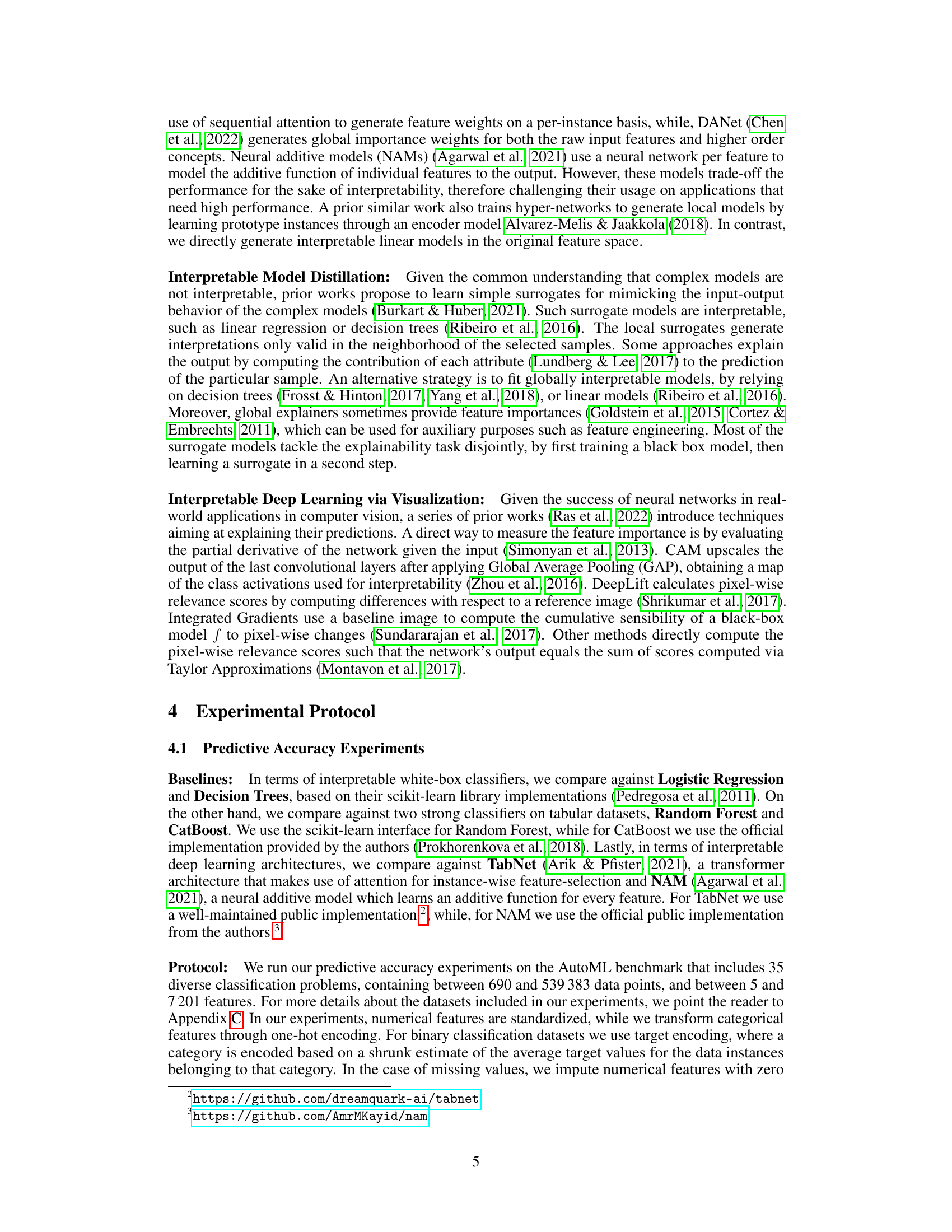
This table shows the feature ranking based on importance for the Census dataset, using several explainable methods (SHAP, Decision Tree, TabNet, CatBoost, and IMN). A lower rank indicates a higher importance for that feature in predicting the target variable. This allows a comparison of how these different methods assess the relative importance of features.
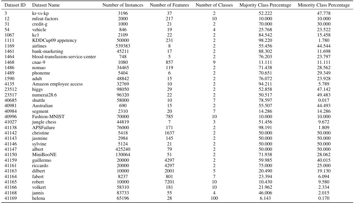
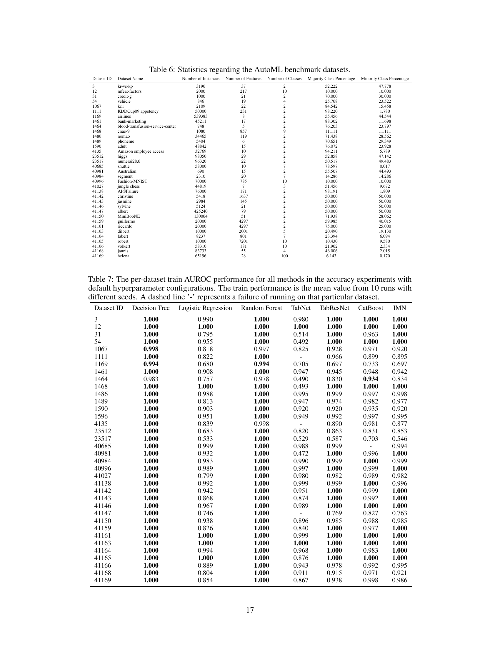
This table provides a statistical overview of the 35 datasets used in the AutoML benchmark experiments. For each dataset, it lists the dataset ID, dataset name, number of instances, number of features, number of classes, majority class percentage, and minority class percentage. The table offers a comprehensive summary of the characteristics of the datasets used in the study’s predictive accuracy experiments. This information is crucial for understanding the context and generalizability of the experimental results.
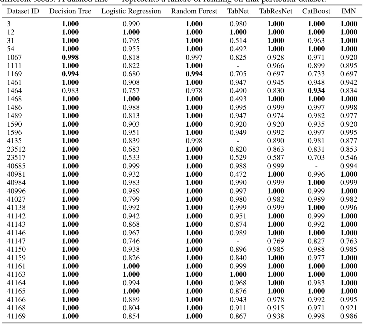
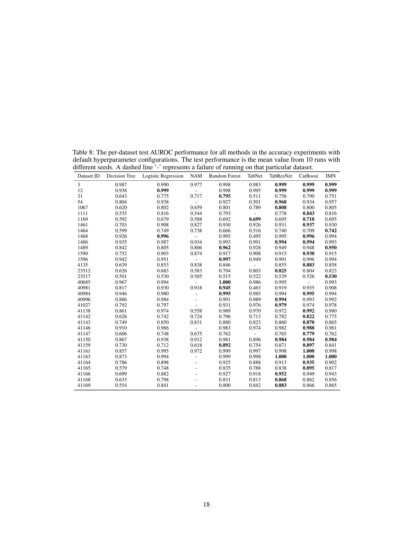
This table shows the test AUROC (Area Under the Receiver Operating Characteristic curve) for multiple classification models on various datasets. The models compared include Decision Tree, Logistic Regression, NAM, Random Forest, TabNet, TabResNet, CatBoost, and IMN. The AUROC values represent the average performance over 10 runs with different random seeds, offering a robust comparison of model performance. A dash indicates that a specific model failed to produce a result for a particular dataset. This table is part of the analysis comparing different models’ predictive accuracy on multiple datasets using default hyperparameters.

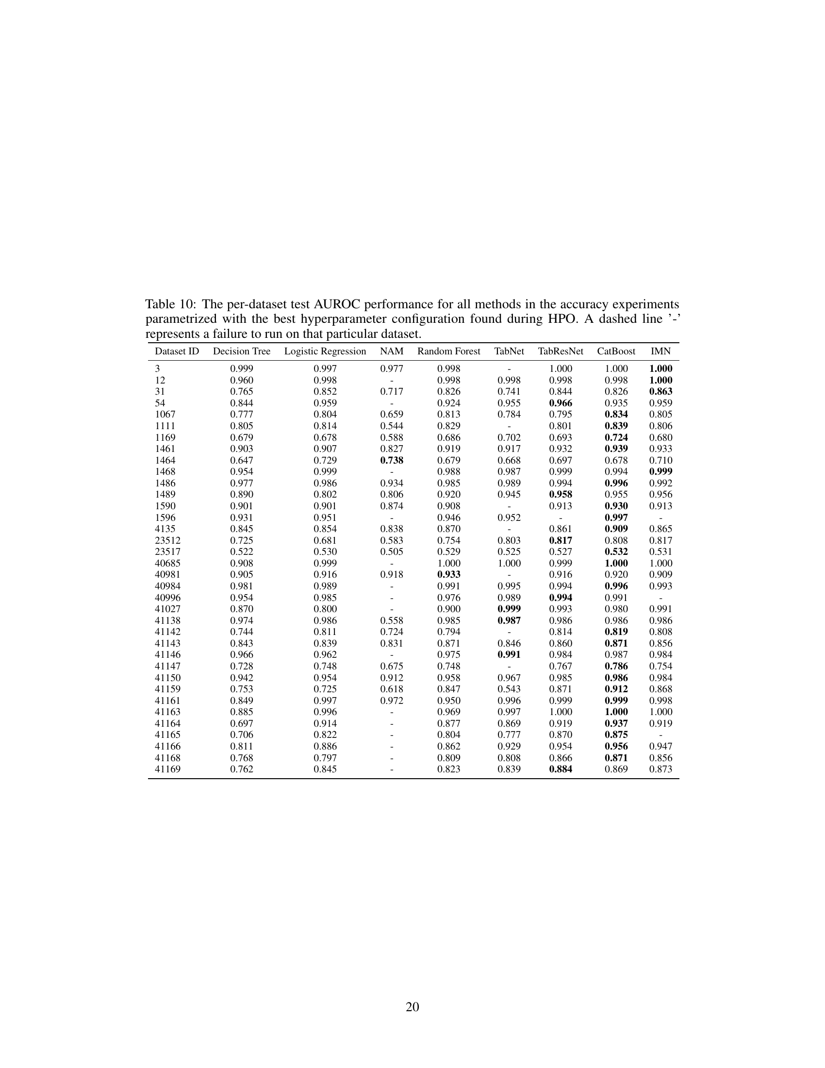
This table presents the test AUROC (Area Under the Receiver Operating Characteristic curve) performance for different classification models on various datasets. The results are averaged over 10 runs with different random seeds, to provide a measure of robustness. A dash indicates that the model failed to run on that specific dataset. The models compared include Decision Tree, Logistic Regression, NAM, Random Forest, TabNet, TabResNet, CatBoost, and IMN (Interpretable Mesomorphic Network). The table helps to evaluate the predictive accuracy of different methods on a diverse range of datasets, using a standard performance metric.
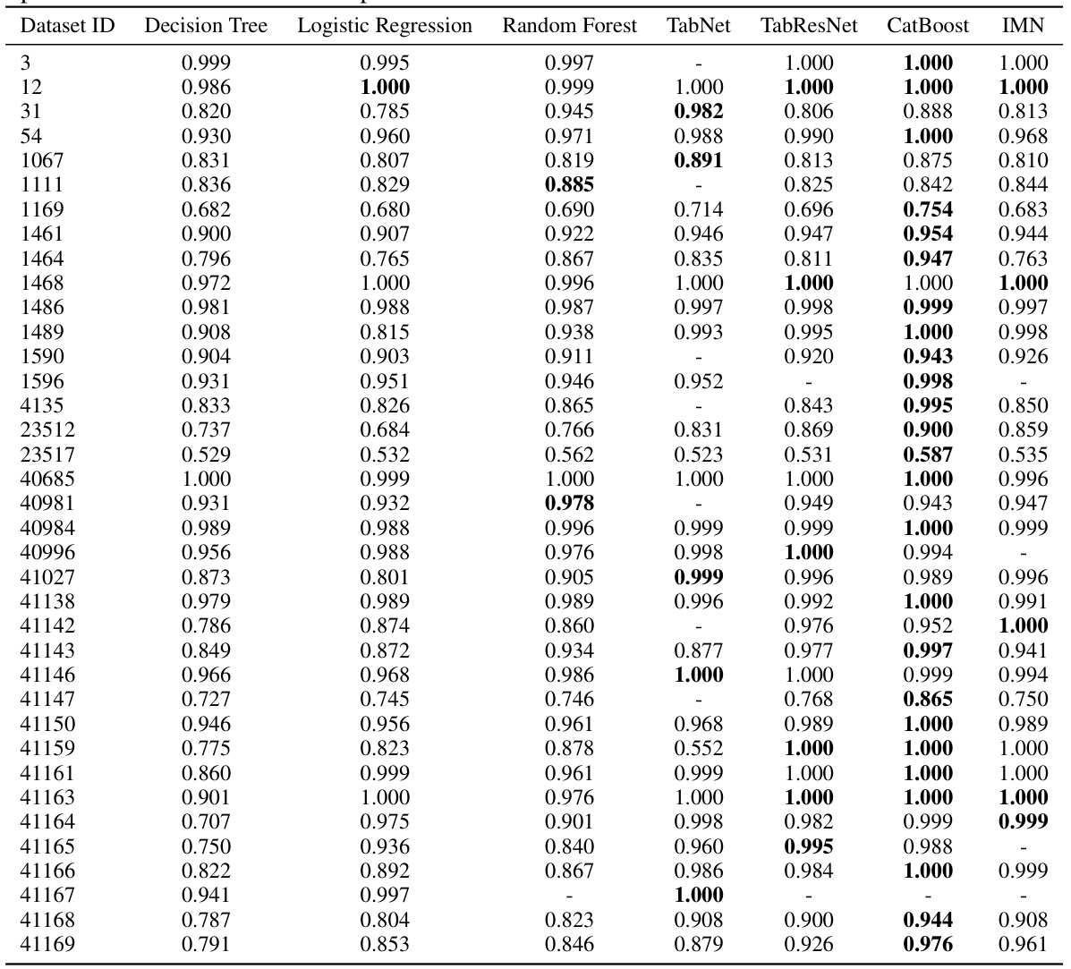
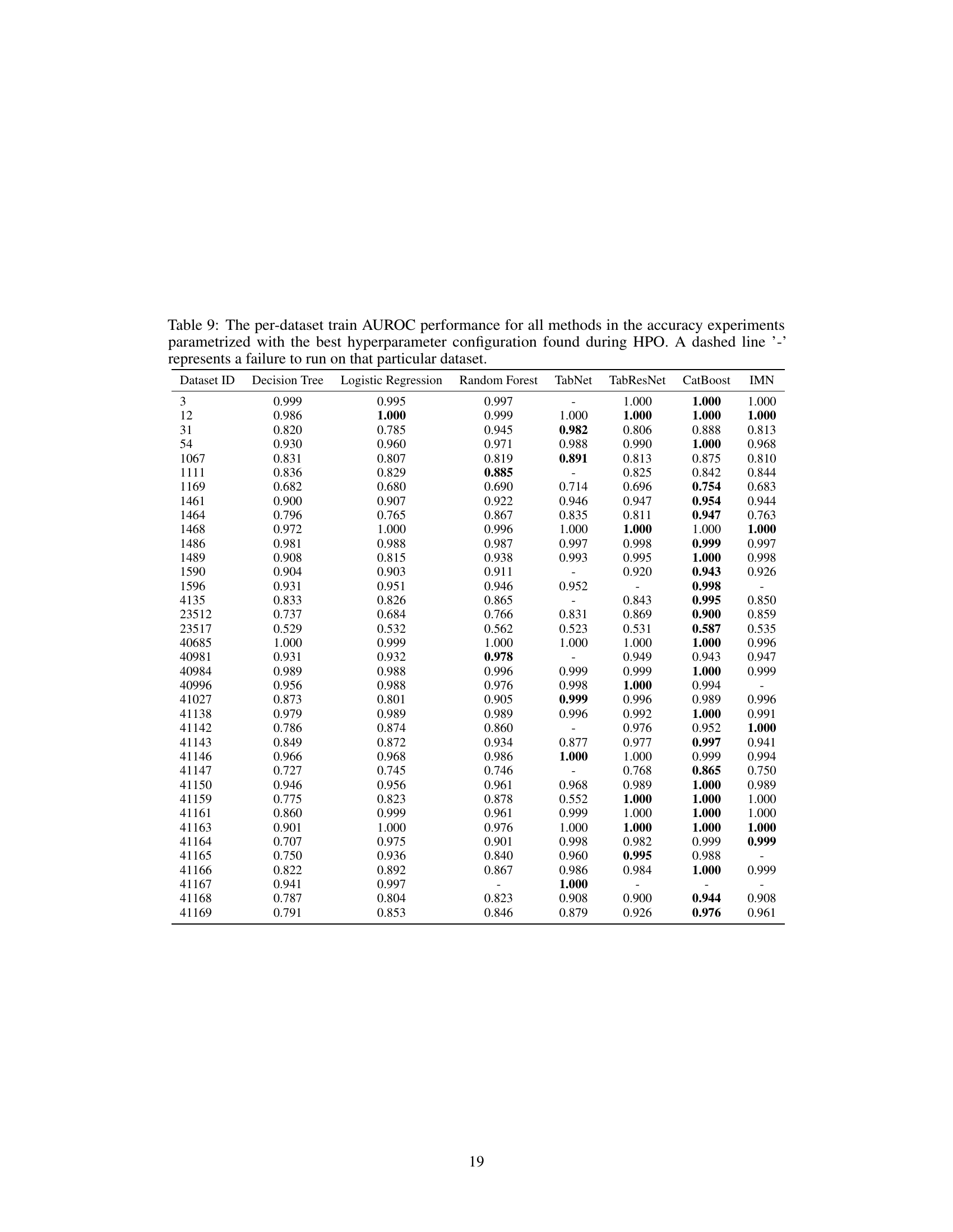
This table presents the test AUROC (Area Under the Receiver Operating Characteristic curve) performance of several classification methods on 35 different datasets from the AutoML benchmark. Each method’s AUROC is the average across 10 runs with different random seeds. The results show the predictive accuracy of different models, including Decision Tree, Logistic Regression, Random Forest, TabNet, TabResNet, CatBoost, and the proposed IMN (Interpretable Mesomorphic Network) model. A ‘-’ indicates that a specific method failed to run on a particular dataset.

This table presents the test AUROC (Area Under the Receiver Operating Characteristic curve) performance of different machine learning methods on 35 diverse datasets. The methods compared include Decision Tree, Logistic Regression, NAM, Random Forest, TabNet, TabResNet, CatBoost, and IMN (Interpretable Mesomorphic Network). The AUROC scores represent the average performance across ten runs with varying random seeds, providing a measure of model robustness. A dash indicates that a particular method failed to complete the experiment for that specific dataset.

This table compares the performance of IMN against other state-of-the-art methods on multiple interpretability metrics. The metrics used are faithfulness, faithfulness (ROAR), infidelity, monotonicity (ROAR), and Shapley Correlation. The results are generated from three datasets within the XAI Benchmark.

This table presents the accuracy of local hyperplanes generated by the IMN model for varying numbers of neighboring points. It shows how well the linear model generated for a single data point generalizes to its neighbors. The results demonstrate the local accuracy of the learned linear models.

This table compares the performance of the proposed IMN model against eight state-of-the-art explainability methods across three datasets from the XAI Benchmark. The comparison uses five interpretability metrics: Faithfulness, Monotonicity, Infidelity, and Shapley Correlation. The table shows the numerical results for each method and metric on each dataset, allowing for a direct comparison of the IMN’s interpretability against existing techniques.
This table presents the accuracy of local hyperplanes generated by the IMN model for varying numbers of neighboring points. It demonstrates the model’s ability to generate accurate linear classifiers not only for a specific data point but also for its neighboring points, showcasing its local accuracy and interpretability.
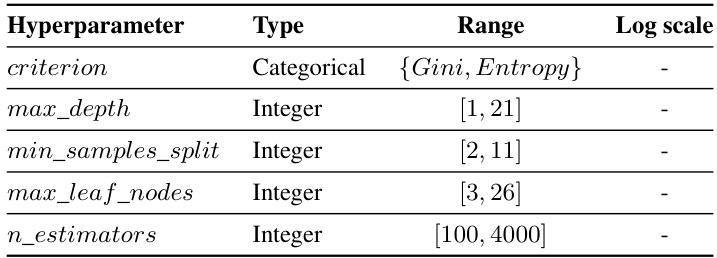
This table shows the accuracy of the local hyperplanes generated by the IMN model for different numbers of neighboring points. The accuracy is evaluated by classifying the neighborhood of each point using the hyperplane generated for that point. The results indicate that the IMN model generates accurate local hyperplanes for the neighborhood of points, with an accuracy of 0.84 for 10 neighbors and 0.77 for 200 neighbors.
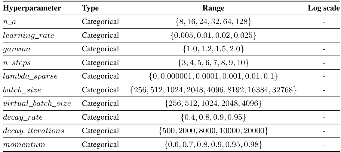
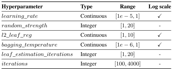
This table presents the hyperparameter search space used for tuning the TabNet model during the experiments. Each hyperparameter is listed along with its data type (categorical or continuous) and the range of values considered. Note that the
log_scalecolumn indicates whether the logarithmic scale was used for the hyperparameter’s range. This information is crucial for understanding the hyperparameter optimization process and how the TabNet model was tuned for optimal performance.
Full paper#


