TL;DR#
Improving the generalization ability of machine learning models is a significant research focus. Sharpness Aware Minimization (SAM) has emerged as a promising technique, but its effectiveness diminishes as model size increases. This study reveals that standard SAM primarily affects the final layer in wide networks. This leads to a critical limitation: hyperparameters optimized for smaller models may not transfer effectively to larger models. This limits efficiency.
To overcome this challenge, the researchers propose µP² (Maximal Update and Perturbation Parameterization). This novel parameterization incorporates layerwise perturbation scaling, ensuring that all layers contribute to the feature learning process. Through rigorous theoretical analysis and experiments, µP² is shown to successfully transfer optimal hyperparameters (learning rate and perturbation radius) across varying model sizes, resulting in significantly improved generalization performance. The paper also provides a versatile condition for µP² application across diverse architectures and SAM variants, enhancing its applicability and impact.
Key Takeaways#
Why does it matter?#
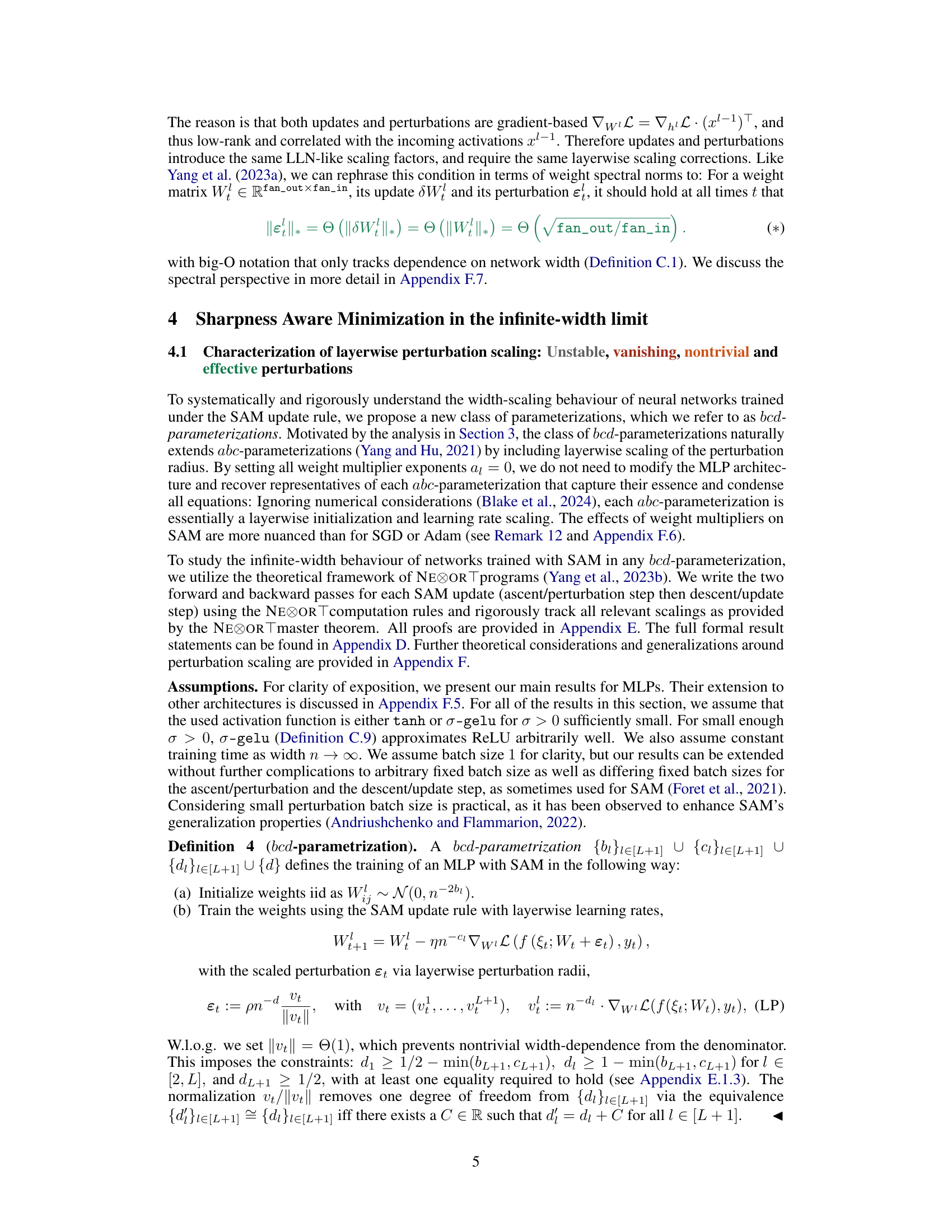
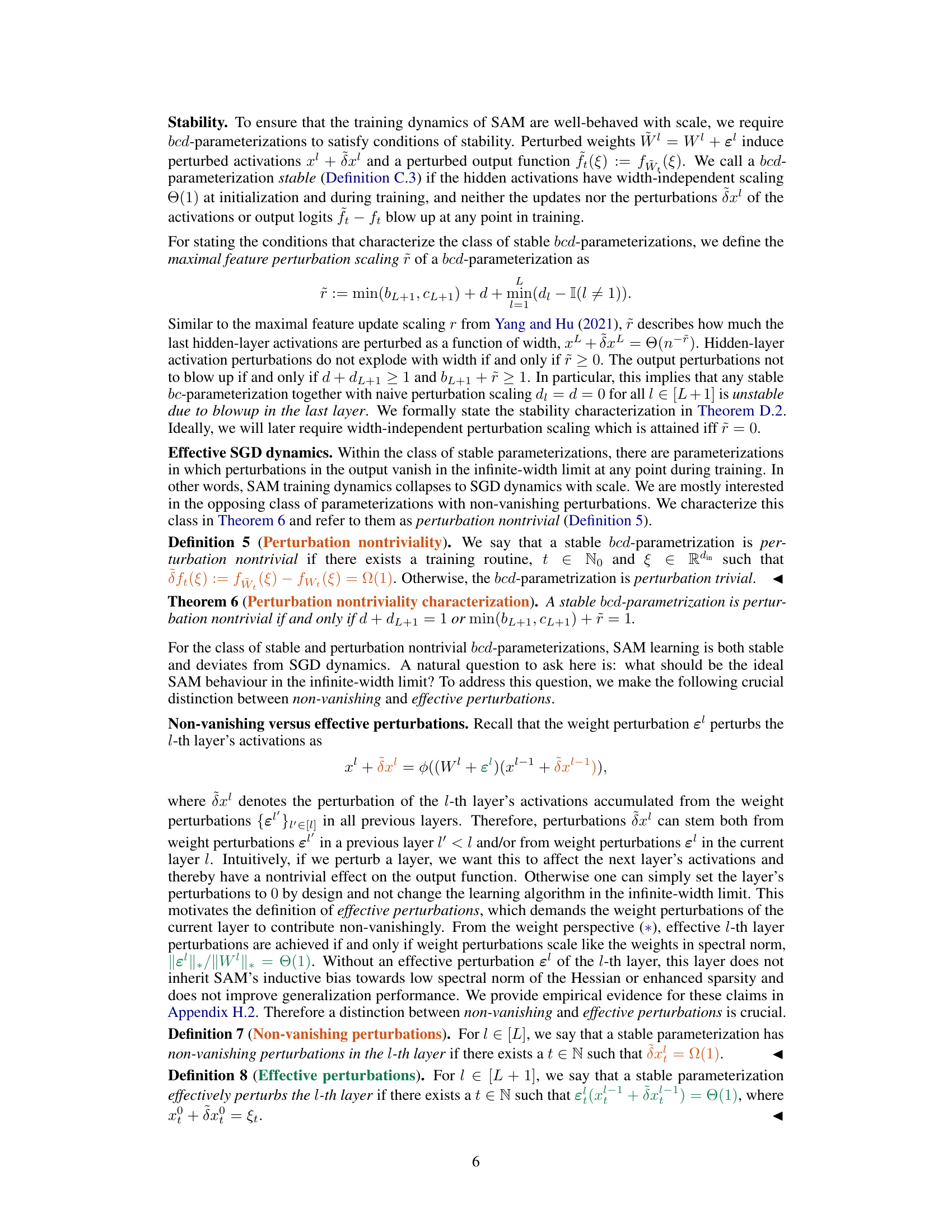
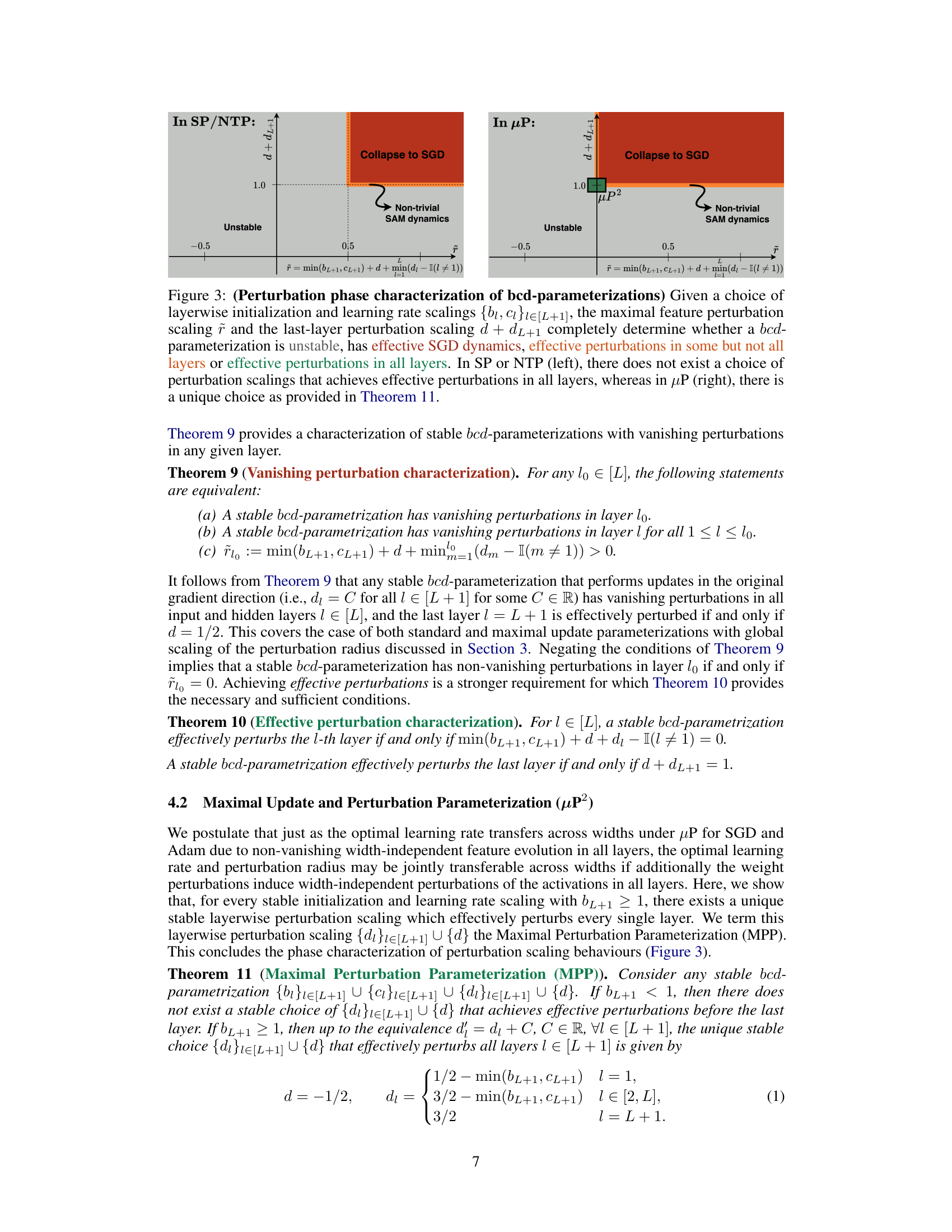
This paper is crucial because it addresses the scalability challenges of Sharpness Aware Minimization (SAM), a popular technique for improving model generalization. By providing a theoretical understanding of SAM’s behavior in wide neural networks and introducing µP², the paper offers practical guidelines for applying SAM to large models, a significant step toward improving the performance of state-of-the-art AI systems. Furthermore, it provides a versatile condition applicable to various SAM variants and other architectures. This is highly relevant to current research trends in large-scale model training and generalization.
Visual Insights#
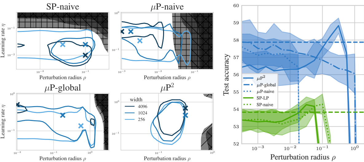
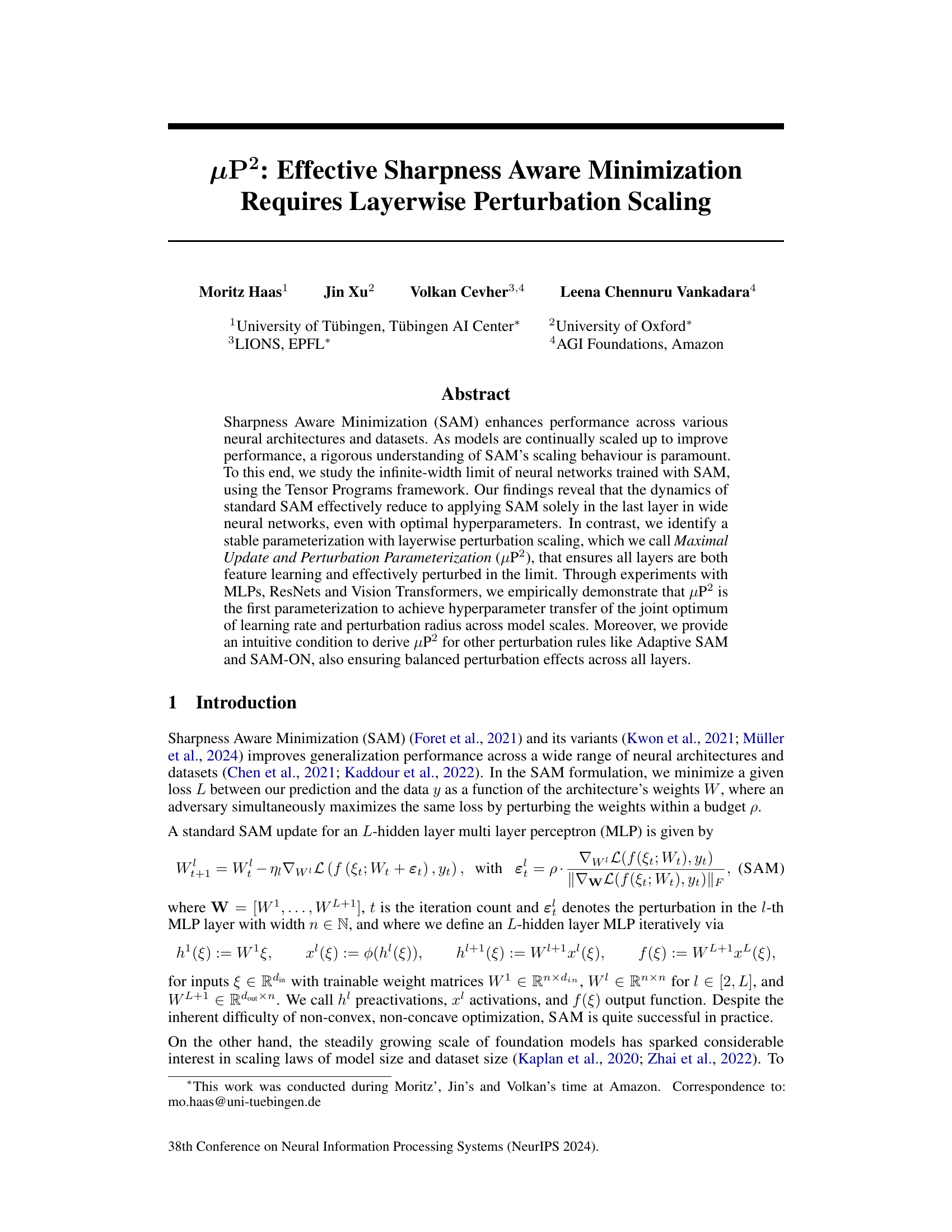
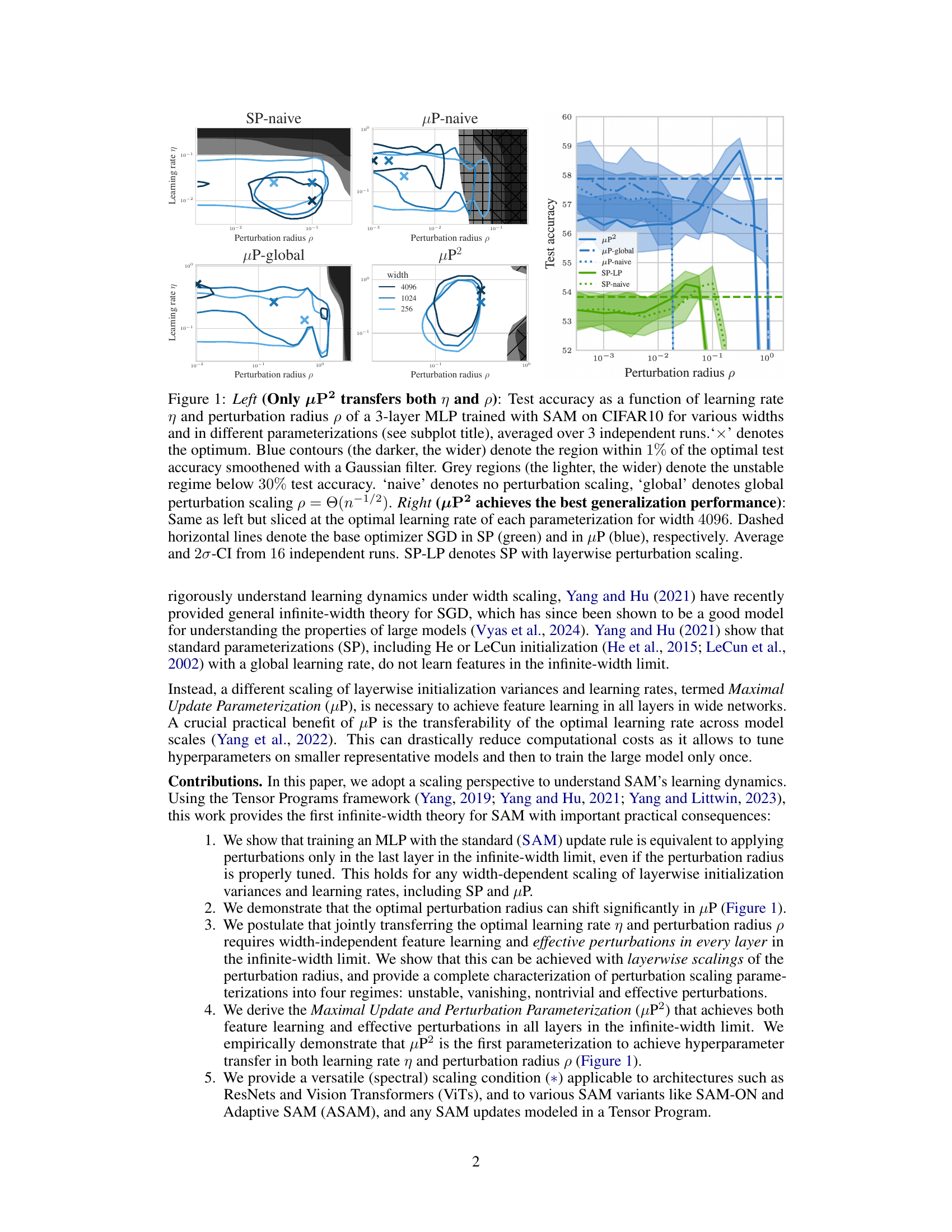
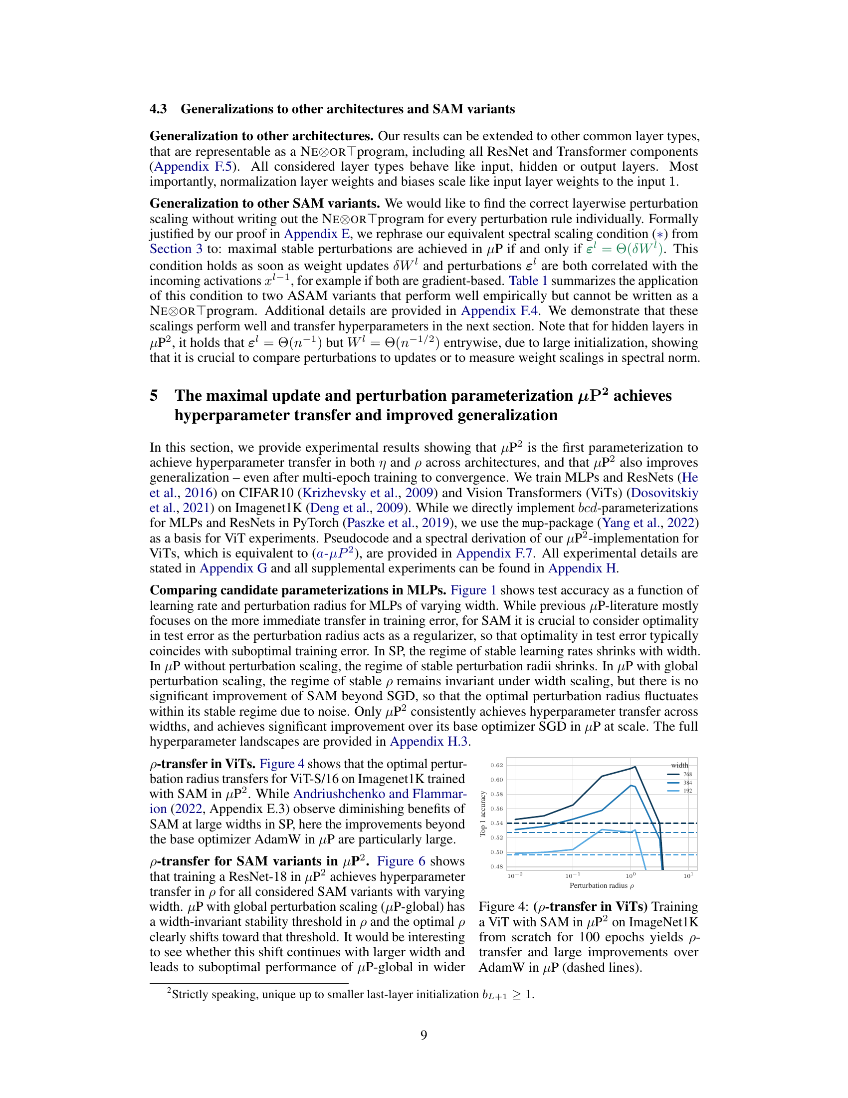
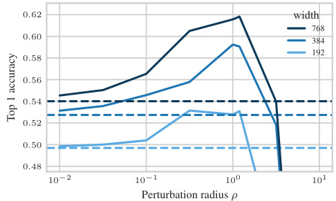
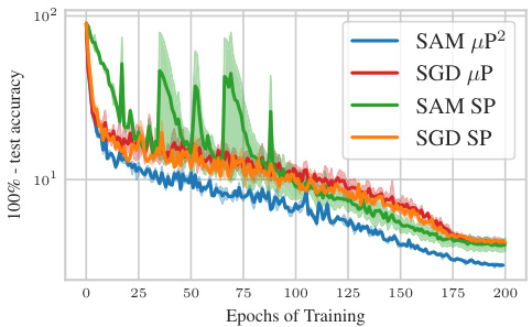
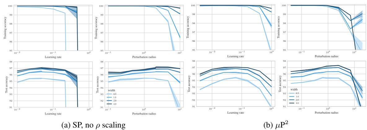
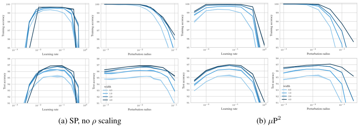
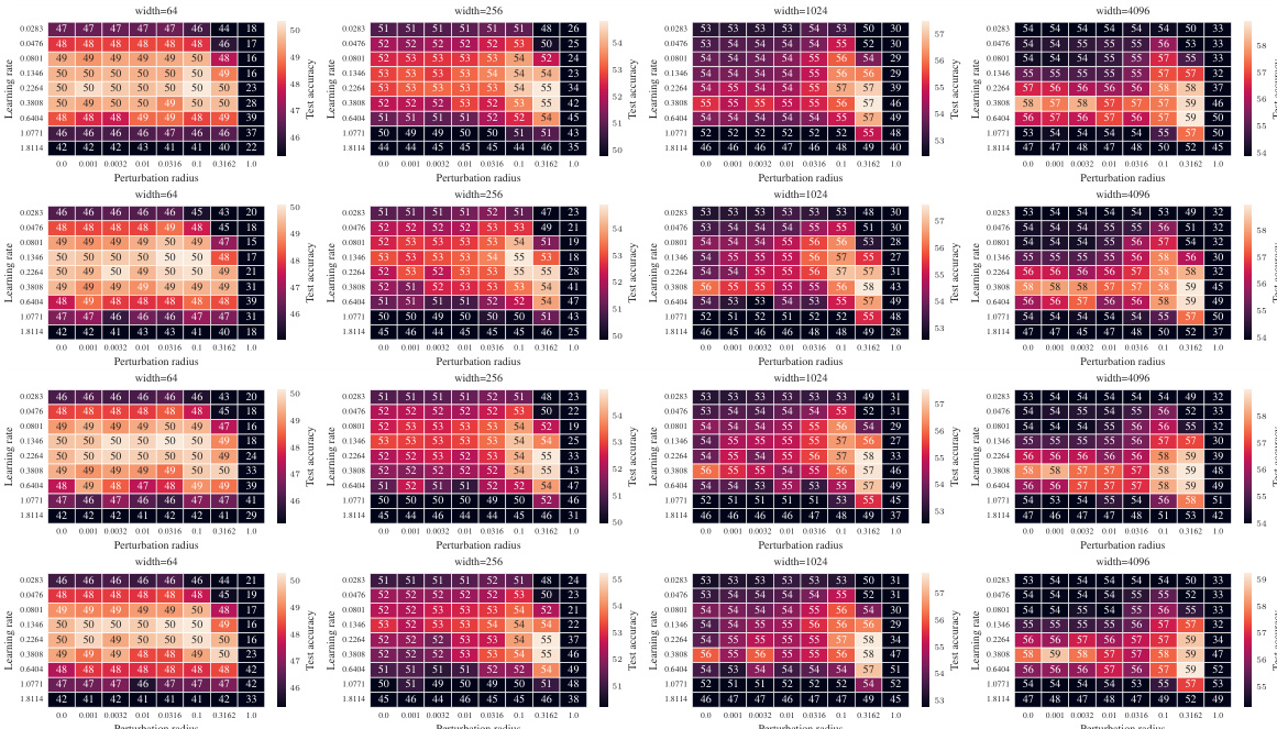
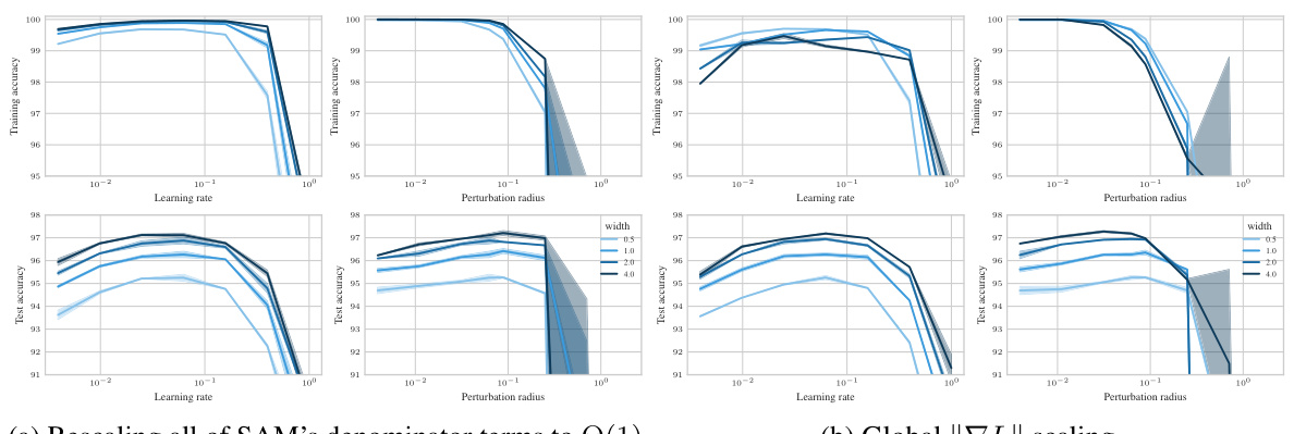
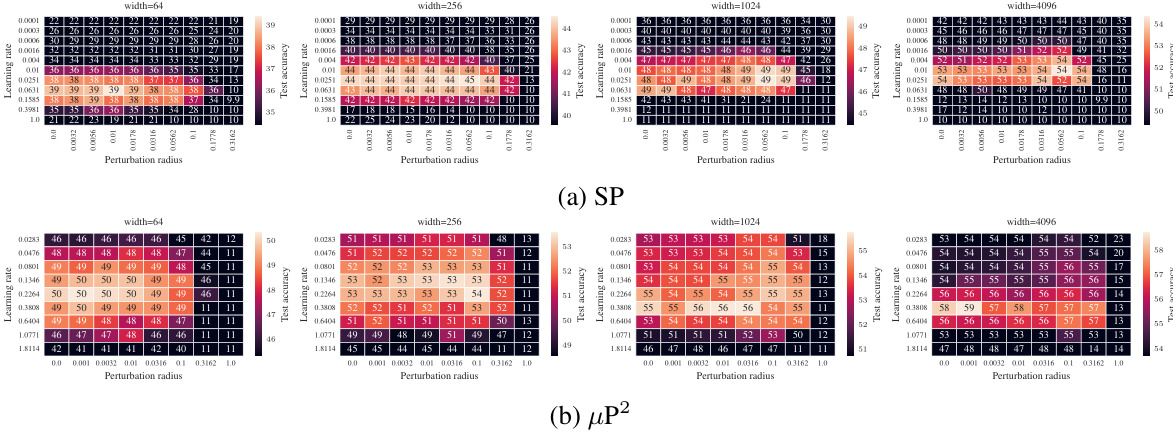
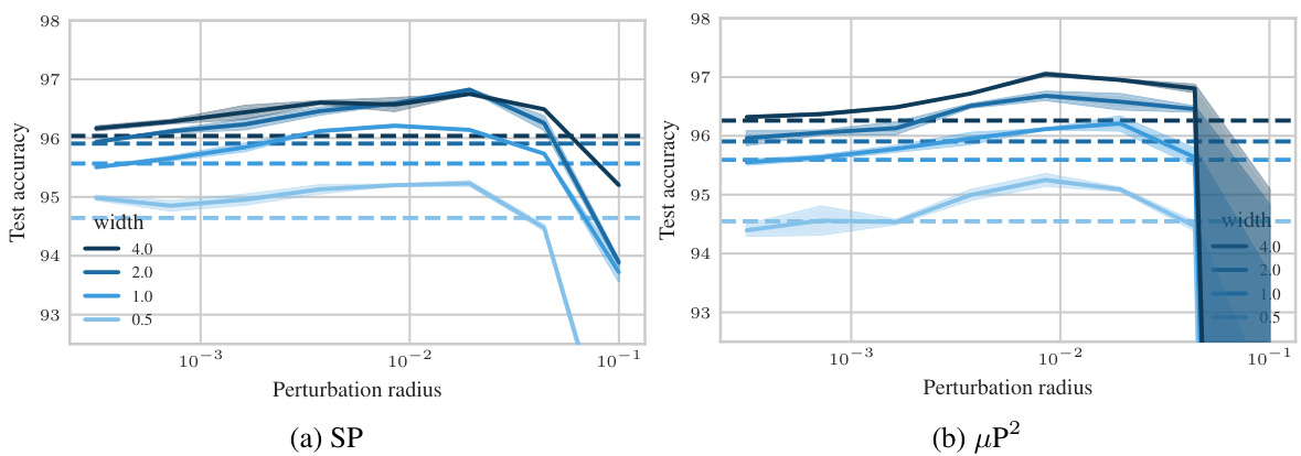
🔼 This figure shows the test accuracy of a 3-layer Multi-Layer Perceptron (MLP) trained on CIFAR10 using Sharpness Aware Minimization (SAM) with different parameterizations. The left panel shows a contour plot of test accuracy as a function of learning rate (η) and perturbation radius (ρ) for various MLP widths. It highlights that only the µP² parameterization allows for transferability of optimal hyperparameters across different model widths. The right panel shows a slice of the left panel at the optimal learning rate for each parameterization and width 4096, further emphasizing the superior generalization performance of µP². The figure demonstrates the importance of layerwise perturbation scaling for achieving consistent performance across different model scales.
read the caption
Figure 1: Left (Only µP² transfers both η and p): Test accuracy as a function of learning rate η and perturbation radius p of a 3-layer MLP trained with SAM on CIFAR10 for various widths and in different parameterizations (see subplot title), averaged over 3 independent runs. ‘×’ denotes the optimum. Blue contours (the darker, the wider) denote the region within 1% of the optimal test accuracy smoothened with a Gaussian filter. Grey regions (the lighter, the wider) denote the unstable regime below 30% test accuracy. ‘naive’ denotes no perturbation scaling, ‘global’ denotes global perturbation scaling p = Θ(n-1/2). Right (µP2 achieves the best generalization performance): Same as left but sliced at the optimal learning rate of each parameterization for width 4096. Dashed horizontal lines denote the base optimizer SGD in SP (green) and in µP (blue), respectively. Average and 20-CI from 16 independent runs. SP-LP denotes SP with layerwise perturbation scaling.

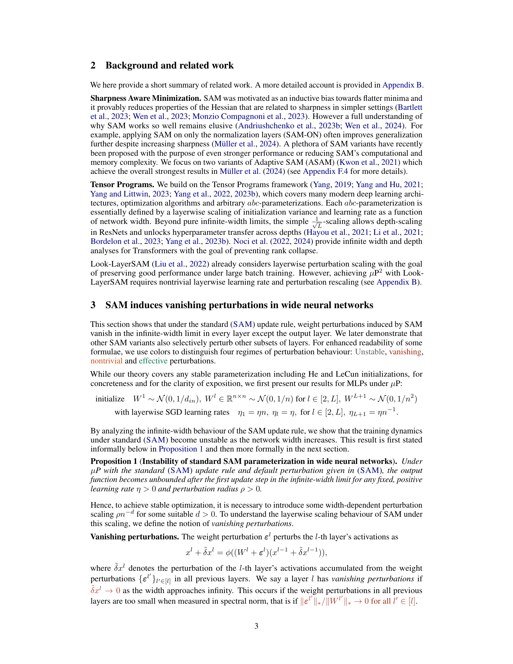
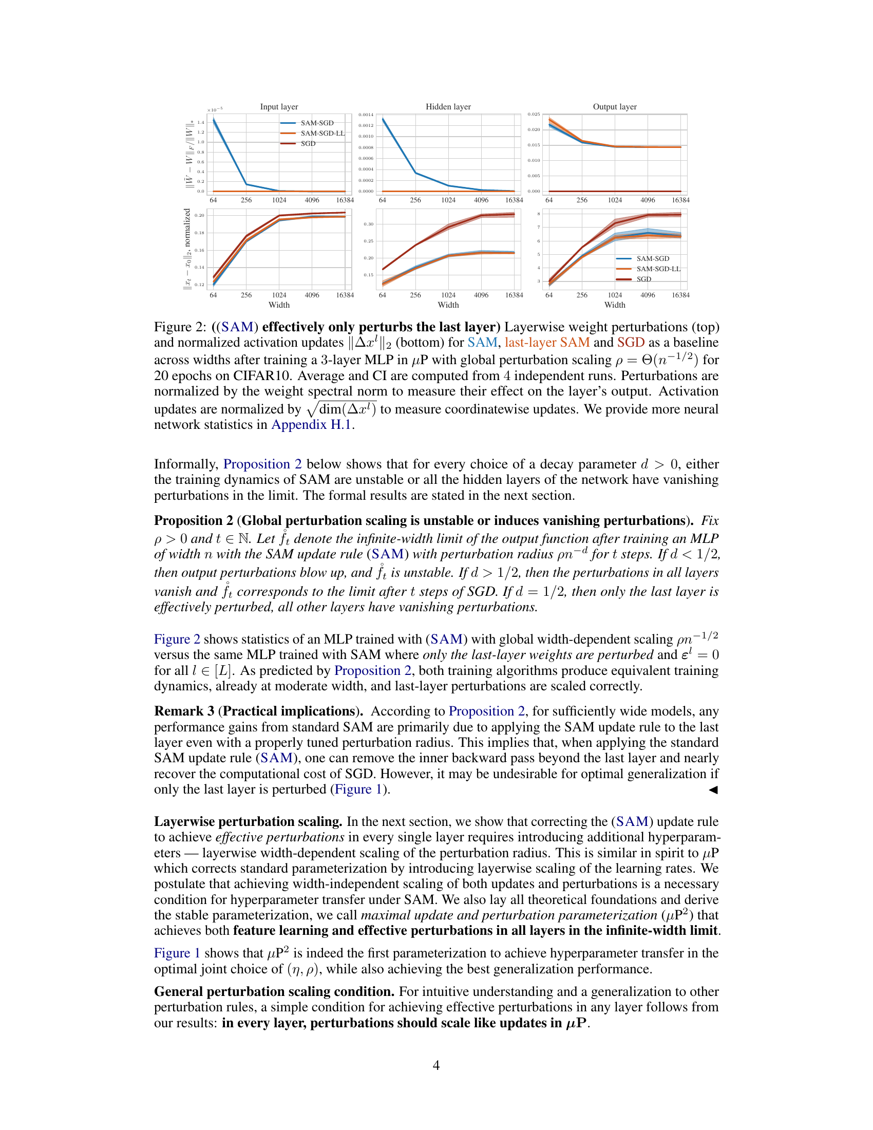
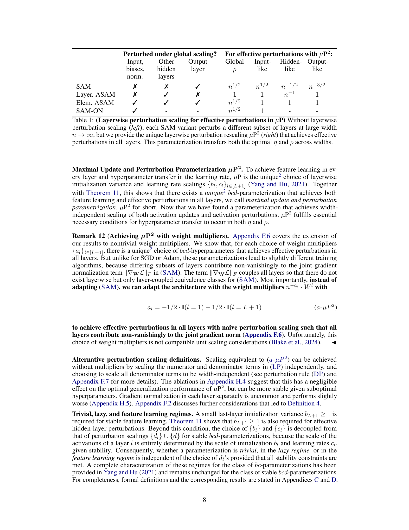
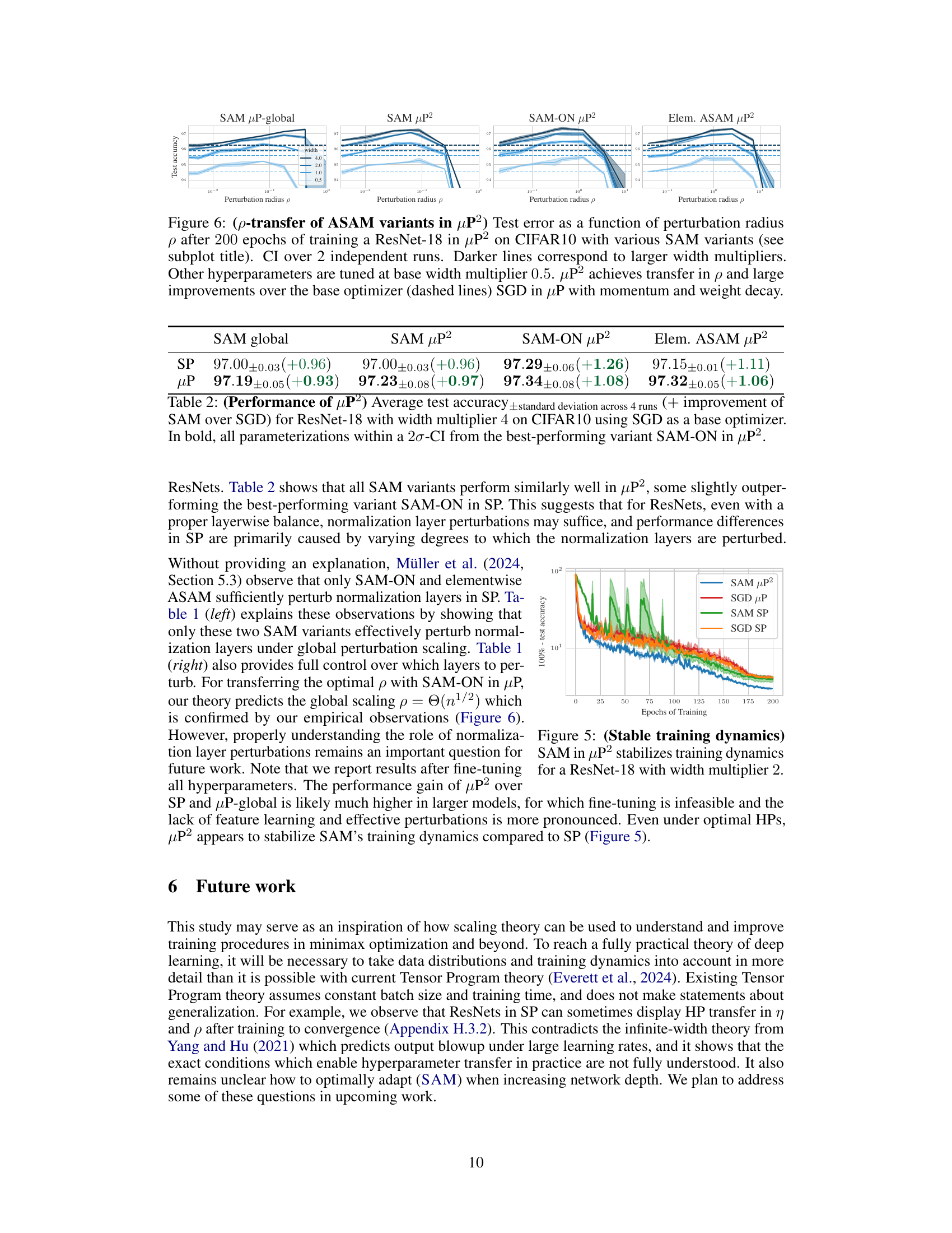
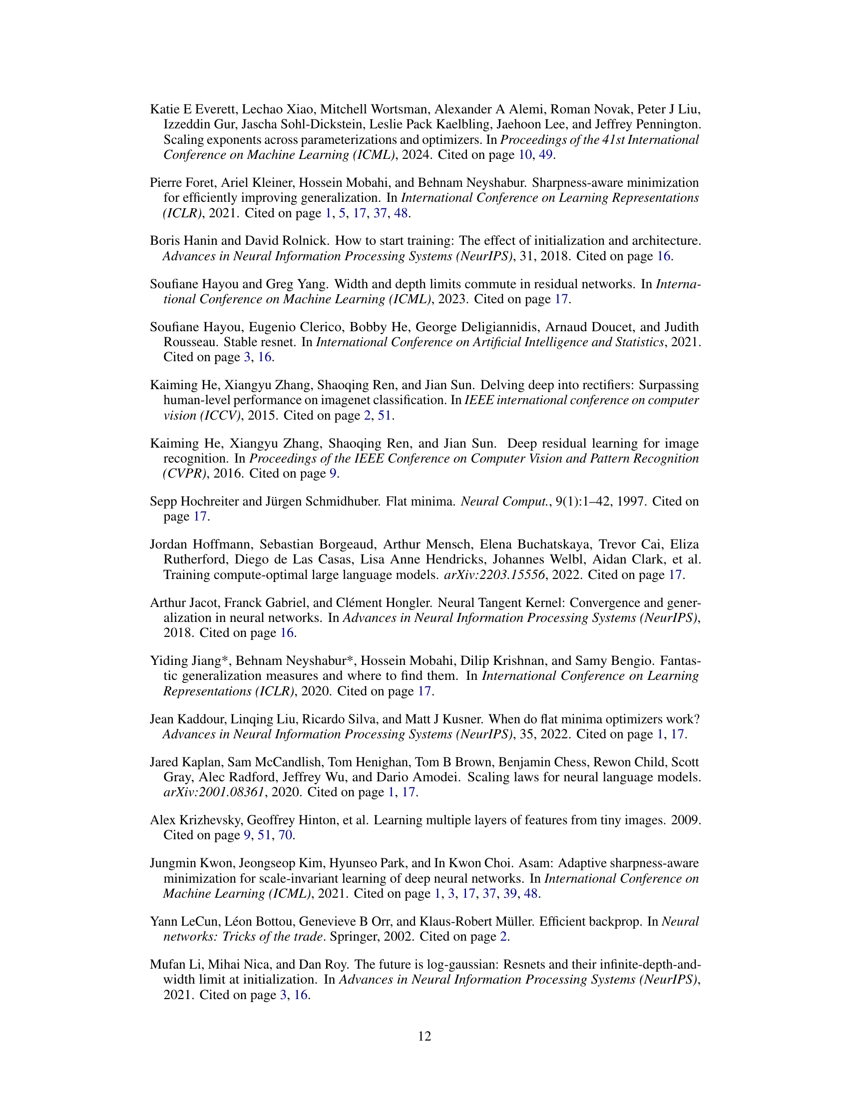
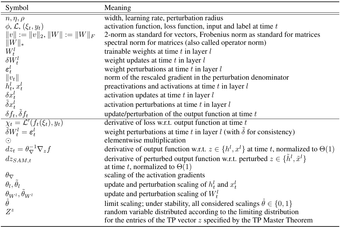
🔼 This table summarizes which layers are perturbed by different SAM variants under different parameterizations at large width n→∞. The left side shows the layers that are perturbed under global perturbation scaling without layerwise scaling. The right side shows which layers are effectively perturbed under µP² with layerwise perturbation scaling. The table highlights that µP² uniquely achieves effective perturbations in all layers and transfers both optimal learning rate and perturbation radius across model widths.
read the caption
Table 1: (Layerwise perturbation scaling for effective perturbations in µP) Without layerwise perturbation scaling (left), each SAM variant perturbs a different subset of layers at large width n→∞, but we provide the unique layerwise perturbation rescaling µP² (right) that achieves effective perturbations in all layers. This parameterization transfers both the optimal η and p across widths.
In-depth insights#
SAM Scaling Limits#
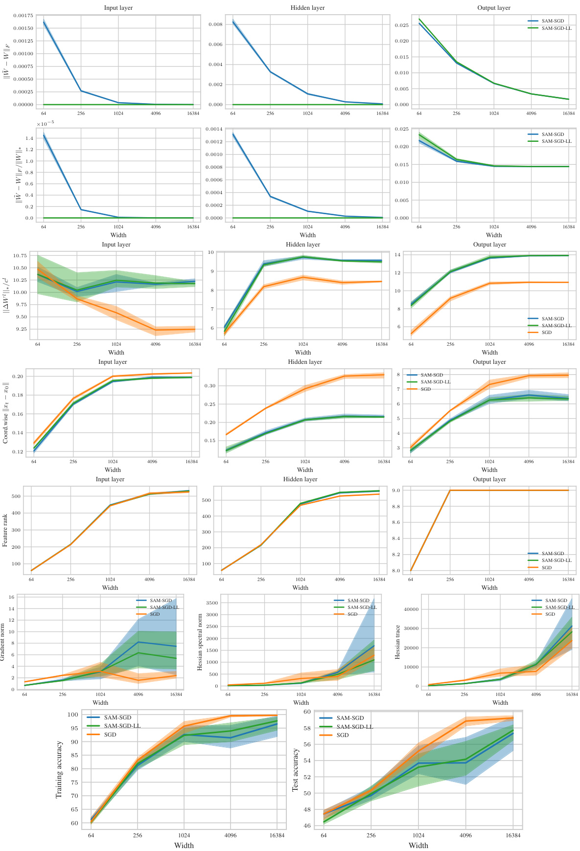
The heading ‘SAM Scaling Limits’ suggests an investigation into the behavior of Sharpness-Aware Minimization (SAM) as model size and complexity increase. A key focus would likely be on identifying limitations in SAM’s effectiveness at scale. This might involve analyzing how SAM’s hyperparameters (learning rate and perturbation radius) need to be adjusted for different model sizes, and exploring scenarios where SAM’s adversarial perturbation becomes ineffective or computationally expensive. The analysis might also consider how SAM interacts with other scaling phenomena, such as the impact of increased data size or model depth. A significant aspect would be determining if SAM’s generalization benefits are maintained in large-scale models, or if alternative optimization strategies become more suitable. Ultimately, understanding SAM’s scaling limits is crucial for developing practical and scalable training methods for increasingly complex deep learning models. The findings would likely lead to improved hyperparameter tuning strategies for SAM in large-scale settings and may even suggest modifications to the algorithm itself to enhance its scalability and performance.
µP² Parameterization#
The µP² parameterization is a novel approach to enhance the performance and scalability of Sharpness Aware Minimization (SAM). It addresses SAM’s limitations in scaling to wider neural networks by introducing layerwise perturbation scaling. Unlike standard SAM, which reduces to a single-layer perturbation in wide networks, µP² ensures that all layers are effectively perturbed, leading to improved hyperparameter transferability and generalization. The key innovation is applying layer-wise scaling factors to the perturbation radius, balancing the perturbation effects across all layers. This method is theoretically grounded and empirically validated, demonstrating significant improvements in performance and hyperparameter transferability across diverse model architectures. µP² represents a crucial step towards more efficient and scalable training of large-scale neural networks with SAM, enabling better hyperparameter optimization across various model sizes and datasets.
Infinite-Width Theory#
The concept of ‘Infinite-Width Theory’ in the context of neural networks centers on analyzing network behavior as the number of neurons in each layer approaches infinity. This theoretical framework simplifies the analysis of complex network dynamics, offering valuable insights into generalization, optimization, and other key aspects. A central benefit is the transition from complex, high-dimensional weight spaces to simpler, often deterministic, dynamics. This simplification allows researchers to derive theoretical guarantees and understand fundamental properties that might be obscured by finite-width complexities. For example, infinite-width analyses can reveal how specific parameterizations or training algorithms affect the model’s ability to learn features or generalize to unseen data. It’s crucial to note that infinite-width results serve as approximations for very wide, but finite-width, networks. This means that while infinite-width theory provides valuable insights into the underlying mechanisms, the actual behavior of real-world, finite-width networks may deviate to some extent. Therefore, results from infinite-width analyses should always be interpreted carefully and considered alongside empirical evaluations.
Hyperparameter Transfer#
The concept of “Hyperparameter Transfer” in the context of this research paper centers on the ability to reuse optimal hyperparameters (like learning rate and perturbation radius) across models of varying sizes (widths). Standard approaches fail to achieve this due to changes in the model’s learning dynamics as the width scales. The paper argues that this limitation stems from the interaction of the SAM (Sharpness Aware Minimization) update rule and the model’s parameterization. They introduce a new parameterization, µP², which through layerwise perturbation scaling, ensures that all layers remain effectively perturbed in the infinite width limit. This crucial element enables the transferability of optimal hyperparameters, significantly reducing computational costs associated with hyperparameter tuning for large models. The authors experimentally validate µP², demonstrating its effectiveness across different architectures (MLPs, ResNets, ViTs) and SAM variants, highlighting its practicality and potential as a significant step in efficient deep learning model training.
Future Research#
The paper’s “Future Work” section suggests several promising avenues for extending this research. Scaling laws are mentioned, implying a need to incorporate data distribution and training dynamics beyond the current infinite-width model. Hyperparameter transferability, a key achievement of the current work, should be further explored, particularly how it behaves in practice with very large models. The interaction between different SAM variants and their optimal parameterization warrants investigation. There’s also a call for a deeper understanding of the roles of normalization layers within the broader SAM framework, and how perturbation scaling interacts with those normalization dynamics. Finally, the authors propose extending the theory to deeper networks, where the assumptions of the current framework may not hold. This comprehensive future work plan points towards a more robust and practically applicable understanding of SAM’s behavior in larger-scale settings.
More visual insights#
More on figures
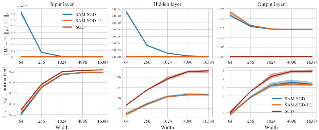
🔼 This figure shows the results of experiments on a 3-layer MLP trained with SAM on CIFAR10 dataset. The experiments test different parameterizations of SAM, varying learning rate (η) and perturbation radius (ρ) for MLPs of different widths. The left panel shows a contour plot illustrating the test accuracy across various learning rates and perturbation radii, highlighting the optimal parameter region for each configuration. The right panel presents a slice through the optimal learning rate for a width of 4096, emphasizing the superior generalization performance of the proposed µP² parameterization.
read the caption
Figure 1: Left (Only µP² transfers both η and p): Test accuracy as a function of learning rate η and perturbation radius p of a 3-layer MLP trained with SAM on CIFAR10 for various widths and in different parameterizations (see subplot title), averaged over 3 independent runs. ‘×’ denotes the optimum. Blue contours (the darker, the wider) denote the region within 1% of the optimal test accuracy smoothened with a Gaussian filter. Grey regions (the lighter, the wider) denote the unstable regime below 30% test accuracy. ‘naive’ denotes no perturbation scaling, ‘global’ denotes global perturbation scaling p = Θ(n-1/2). Right (µP2 achieves the best generalization performance): Same as left but sliced at the optimal learning rate of each parameterization for width 4096. Dashed horizontal lines denote the base optimizer SGD in SP (green) and in µP (blue), respectively. Average and 20-CI from 16 independent runs. SP-LP denotes SP with layerwise perturbation scaling.

🔼 This figure empirically demonstrates the performance of different parameterizations of SAM across various model widths. The left panel shows a contour plot illustrating the test accuracy as a function of the learning rate and perturbation radius for a 3-layer MLP trained on CIFAR10. It highlights that only the proposed µP² parameterization allows for transfer of optimal hyperparameters (learning rate and perturbation radius) across different model widths. The right panel shows the same data but sliced at the optimal learning rate for each parameterization, further emphasizing µP²’s superior generalization performance.
read the caption
Figure 1: Left (Only µP² transfers both η and p): Test accuracy as a function of learning rate η and perturbation radius p of a 3-layer MLP trained with SAM on CIFAR10 for various widths and in different parameterizations (see subplot title), averaged over 3 independent runs. ‘×’ denotes the optimum. Blue contours (the darker, the wider) denote the region within 1% of the optimal test accuracy smoothened with a Gaussian filter. Grey regions (the lighter, the wider) denote the unstable regime below 30% test accuracy. ‘naive’ denotes no perturbation scaling, ‘global’ denotes global perturbation scaling p = Θ(n-1/2). Right (µP2 achieves the best generalization performance): Same as left but sliced at the optimal learning rate of each parameterization for width 4096. Dashed horizontal lines denote the base optimizer SGD in SP (green) and in µP (blue), respectively. Average and 20-CI from 16 independent runs. SP-LP denotes SP with layerwise perturbation scaling.
🔼 The figure shows the test accuracy of a 3-layer Multilayer Perceptron (MLP) trained on CIFAR10 using different parameterizations of Sharpness Aware Minimization (SAM). The left panel shows a heatmap depicting test accuracy across various learning rates (η) and perturbation radii (ρ) for different network widths and parameterizations (SP-naive, µP-naive, µP-global, µP²). The right panel shows a line graph of the test accuracy at the optimal learning rate for each parameterization, highlighting that µP² achieves the best generalization performance and is the only parameterization where both optimal learning rate (η) and perturbation radius (ρ) transfer across different model widths.
read the caption
Figure 1: Left (Only µP² transfers both η and p): Test accuracy as a function of learning rate η and perturbation radius p of a 3-layer MLP trained with SAM on CIFAR10 for various widths and in different parameterizations (see subplot title), averaged over 3 independent runs. ‘×’ denotes the optimum. Blue contours (the darker, the wider) denote the region within 1% of the optimal test accuracy smoothened with a Gaussian filter. Grey regions (the lighter, the wider) denote the unstable regime below 30% test accuracy. ‘naive’ denotes no perturbation scaling, ‘global’ denotes global perturbation scaling p = Θ(n-1/2). Right (µP² achieves the best generalization performance): Same as left but sliced at the optimal learning rate of each parameterization for width 4096. Dashed horizontal lines denote the base optimizer SGD in SP (green) and in µP (blue), respectively. Average and 20-CI from 16 independent runs. SP-LP denotes SP with layerwise perturbation scaling.

🔼 This figure shows the test accuracy of a 3-layer Multilayer Perceptron (MLP) trained on CIFAR10 using different parameterizations of Sharpness Aware Minimization (SAM). The left panel shows a contour plot illustrating how test accuracy varies with learning rate (η) and perturbation radius (ρ) for different model widths and SAM parameterizations. µP² represents the proposed Maximal Update and Perturbation Parameterization. The right panel shows the same data but sliced at the optimal learning rate for each parameterization and width of 4096, highlighting that µP² achieves the best generalization performance and is the only parameterization where both the optimal learning rate and perturbation radius transfer across different model widths.
read the caption
Figure 1: Left (Only µP² transfers both η and p): Test accuracy as a function of learning rate η and perturbation radius p of a 3-layer MLP trained with SAM on CIFAR10 for various widths and in different parameterizations (see subplot title), averaged over 3 independent runs.'×' denotes the optimum. Blue contours (the darker, the wider) denote the region within 1% of the optimal test accuracy smoothened with a Gaussian filter. Grey regions (the lighter, the wider) denote the unstable regime below 30% test accuracy. ‘naive’ denotes no perturbation scaling, ‘global’ denotes global perturbation scaling p = Θ(n-1/2). Right (µP2 achieves the best generalization performance): Same as left but sliced at the optimal learning rate of each parameterization for width 4096. Dashed horizontal lines denote the base optimizer SGD in SP (green) and in µP (blue), respectively. Average and 20-CI from 16 independent runs. SP-LP denotes SP with layerwise perturbation scaling.
🔼 This figure displays the test accuracy of a 3-layer Multilayer Perceptron (MLP) trained on CIFAR10 using Sharpness Aware Minimization (SAM) with different parameterizations. The left subplot shows test accuracy as a function of learning rate and perturbation radius, highlighting the joint optimal hyperparameters for different model widths. The right subplot shows a slice of this data at the optimal learning rate for each parameterization and width 4096. The results indicate that only µP² achieves transferability of optimal hyperparameters across model widths, which shows that µP² is the most effective parameterization for SAM.
read the caption
Figure 1: Left (Only µP² transfers both η and p): Test accuracy as a function of learning rate η and perturbation radius p of a 3-layer MLP trained with SAM on CIFAR10 for various widths and in different parameterizations (see subplot title), averaged over 3 independent runs. ‘×’ denotes the optimum. Blue contours (the darker, the wider) denote the region within 1% of the optimal test accuracy smoothened with a Gaussian filter. Grey regions (the lighter, the wider) denote the unstable regime below 30% test accuracy. ‘naive’ denotes no perturbation scaling, ‘global’ denotes global perturbation scaling p = Θ(n-1/2). Right (µP2 achieves the best generalization performance): Same as left but sliced at the optimal learning rate of each parameterization for width 4096. Dashed horizontal lines denote the base optimizer SGD in SP (green) and in µP (blue), respectively. Average and 20-CI from 16 independent runs. SP-LP denotes SP with layerwise perturbation scaling.
🔼 This figure shows the impact of different parameterizations on the test accuracy of a 3-layer Multi-Layer Perceptron (MLP) trained on CIFAR10 dataset using Sharpness Aware Minimization (SAM). The left panel displays a heatmap showing the test accuracy as a function of learning rate (η) and perturbation radius (p) for various MLP widths and different parameterizations (SP-naive, µP-naive, µP-global, and µP²). The right panel shows a slice of the left panel at the optimal learning rate for each parameterization and width 4096, highlighting the superior generalization performance of µP². The figure demonstrates that µP² is the only parameterization that effectively transfers both the optimal learning rate and perturbation radius across different model scales.
read the caption
Figure 1: Left (Only µP² transfers both η and p): Test accuracy as a function of learning rate η and perturbation radius p of a 3-layer MLP trained with SAM on CIFAR10 for various widths and in different parameterizations (see subplot title), averaged over 3 independent runs. ‘×’ denotes the optimum. Blue contours (the darker, the wider) denote the region within 1% of the optimal test accuracy smoothened with a Gaussian filter. Grey regions (the lighter, the wider) denote the unstable regime below 30% test accuracy. ‘naive’ denotes no perturbation scaling, ‘global’ denotes global perturbation scaling p = Θ(n-1/2). Right (µP2 achieves the best generalization performance): Same as left but sliced at the optimal learning rate of each parameterization for width 4096. Dashed horizontal lines denote the base optimizer SGD in SP (green) and in µP (blue), respectively. Average and 20-CI from 16 independent runs. SP-LP denotes SP with layerwise perturbation scaling.
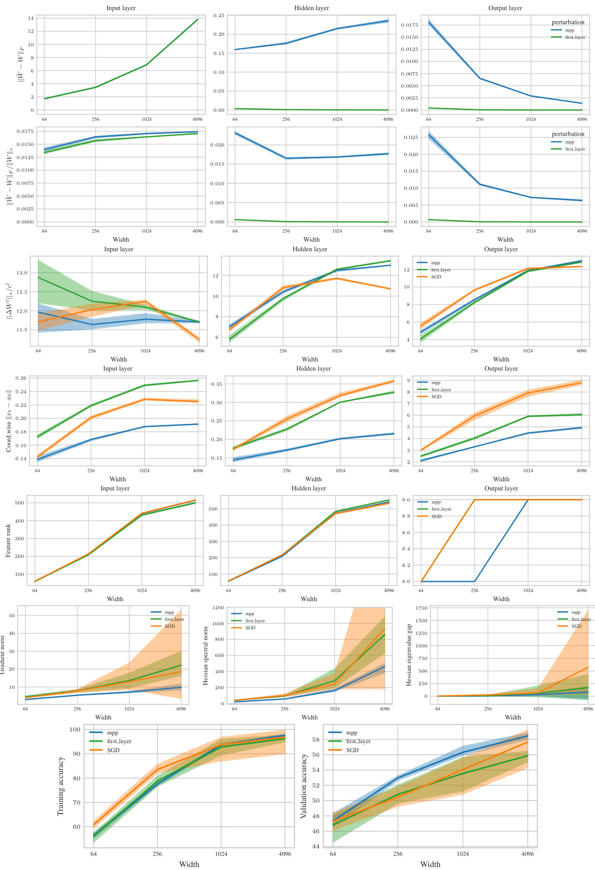
🔼 This figure shows the impact of different parameterizations (SP-naive, µP-naive, µP-global, µP²) on the test accuracy of a 3-layer MLP trained on CIFAR10 with SAM. The left panel shows a heatmap illustrating test accuracy as a function of learning rate (η) and perturbation radius (ρ) for various network widths. It highlights that only the µP² parameterization allows for the joint transfer of optimal η and ρ across different network widths. The right panel shows the test accuracy for each parameterization at the optimal learning rate for a network of width 4096. µP² consistently outperforms other parameterizations, demonstrating its superior generalization ability.
read the caption
Figure 1: Left (Only µP² transfers both η and p): Test accuracy as a function of learning rate η and perturbation radius p of a 3-layer MLP trained with SAM on CIFAR10 for various widths and in different parameterizations (see subplot title), averaged over 3 independent runs. ‘×’ denotes the optimum. Blue contours (the darker, the wider) denote the region within 1% of the optimal test accuracy smoothened with a Gaussian filter. Grey regions (the lighter, the wider) denote the unstable regime below 30% test accuracy. ‘naive’ denotes no perturbation scaling, ‘global’ denotes global perturbation scaling p = Θ(n-1/2). Right (µP2 achieves the best generalization performance): Same as left but sliced at the optimal learning rate of each parameterization for width 4096. Dashed horizontal lines denote the base optimizer SGD in SP (green) and in µP (blue), respectively. Average and 20-CI from 16 independent runs. SP-LP denotes SP with layerwise perturbation scaling.
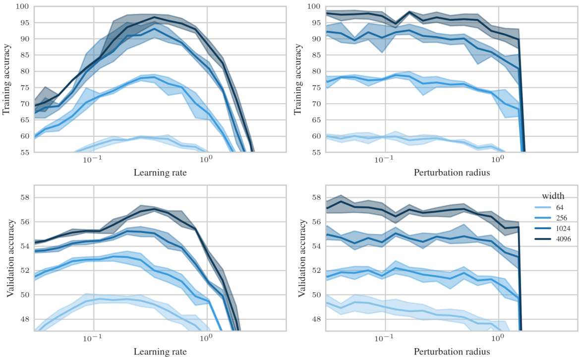
🔼 This figure shows the test accuracy of a 3-layer Multilayer Perceptron (MLP) trained on CIFAR10 dataset using different parameterizations of Sharpness Aware Minimization (SAM). The left panel shows a 2D heatmap of test accuracy as a function of learning rate and perturbation radius for various MLP widths. The right panel shows a 1D slice of the left panel at the optimal learning rate for each parameterization and width 4096. The results demonstrate that only the µP² parameterization achieves both hyperparameter transfer (optimal learning rate and perturbation radius remain similar across model sizes) and the best generalization performance.
read the caption
Figure 1: Left (Only µP² transfers both η and ρ): Test accuracy as a function of learning rate η and perturbation radius ρ of a 3-layer MLP trained with SAM on CIFAR10 for various widths and in different parameterizations (see subplot title), averaged over 3 independent runs. ‘×’ denotes the optimum. Blue contours (the darker, the wider) denote the region within 1% of the optimal test accuracy smoothened with a Gaussian filter. Grey regions (the lighter, the wider) denote the unstable regime below 30% test accuracy. ‘naive’ denotes no perturbation scaling, ‘global’ denotes global perturbation scaling ρ = Θ(n−1/2). Right (µP² achieves the best generalization performance): Same as left but sliced at the optimal learning rate of each parameterization for width 4096. Dashed horizontal lines denote the base optimizer SGD in SP (green) and in µP (blue), respectively. Average and 2σ-CI from 16 independent runs. SP-LP denotes SP with layerwise perturbation scaling.
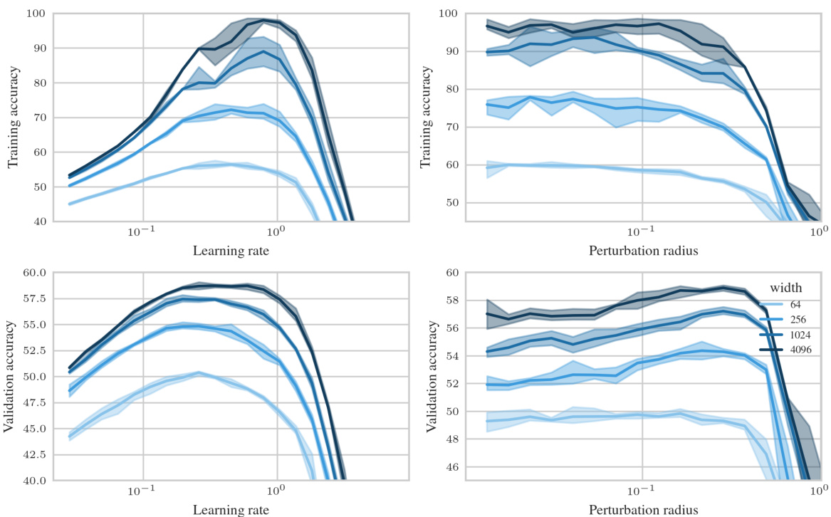
🔼 The figure shows the test accuracy of a 3-layer MLP trained on CIFAR10 using SAM with different parameterizations as a function of learning rate (η) and perturbation radius (ρ). The left panel shows the results across various model widths and parameterizations. The right panel shows the same results but only for the largest model width (4096), with the x-axis showing only the perturbation radius and the lines representing different parameterizations at the optimal learning rate for each. The figure demonstrates that only the µP² parameterization allows for transferability of optimal hyperparameters across model scales. The other parameterizations (SP-naive, µP-naive, µP-global, SP-LP) do not effectively allow this transfer.
read the caption
Figure 1: Left (Only µP² transfers both η and p): Test accuracy as a function of learning rate η and perturbation radius p of a 3-layer MLP trained with SAM on CIFAR10 for various widths and in different parameterizations (see subplot title), averaged over 3 independent runs. ‘×’ denotes the optimum. Blue contours (the darker, the wider) denote the region within 1% of the optimal test accuracy smoothened with a Gaussian filter. Grey regions (the lighter, the wider) denote the unstable regime below 30% test accuracy. ‘naive’ denotes no perturbation scaling, ‘global’ denotes global perturbation scaling p = Θ(n-1/2). Right (µP2 achieves the best generalization performance): Same as left but sliced at the optimal learning rate of each parameterization for width 4096. Dashed horizontal lines denote the base optimizer SGD in SP (green) and in µP (blue), respectively. Average and 20-CI from 16 independent runs. SP-LP denotes SP with layerwise perturbation scaling.
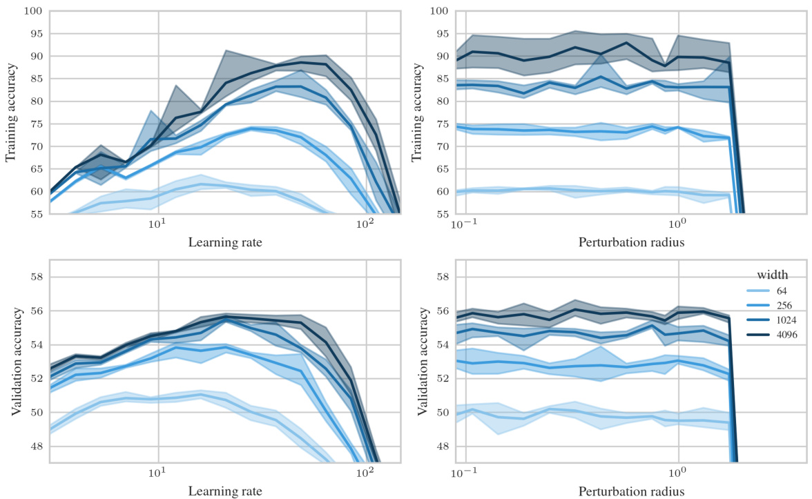
🔼 This figure shows the test accuracy of a 3-layer Multilayer Perceptron (MLP) trained on CIFAR10 using Sharpness Aware Minimization (SAM) with different parameterizations. The left plot shows a contour plot of test accuracy as a function of learning rate (η) and perturbation radius (ρ) for various network widths. The right plot is a slice of the left plot at the optimal learning rate for each parameterization and width 4096. The figure demonstrates that only the proposed µP² parameterization achieves both hyperparameter transfer and optimal generalization performance. The different parameterizations represent different scaling approaches for the perturbation radius.
read the caption
Figure 1: Left (Only µP² transfers both η and p): Test accuracy as a function of learning rate η and perturbation radius p of a 3-layer MLP trained with SAM on CIFAR10 for various widths and in different parameterizations (see subplot title), averaged over 3 independent runs. ‘×’ denotes the optimum. Blue contours (the darker, the wider) denote the region within 1% of the optimal test accuracy smoothened with a Gaussian filter. Grey regions (the lighter, the wider) denote the unstable regime below 30% test accuracy. ‘naive’ denotes no perturbation scaling, ‘global’ denotes global perturbation scaling p = Θ(n-1/2). Right (µP2 achieves the best generalization performance): Same as left but sliced at the optimal learning rate of each parameterization for width 4096. Dashed horizontal lines denote the base optimizer SGD in SP (green) and in µP (blue), respectively. Average and 20-CI from 16 independent runs. SP-LP denotes SP with layerwise perturbation scaling.

🔼 This figure shows the effect of different parameterizations on the test accuracy of a 3-layer MLP trained on CIFAR10 using SAM. It compares four parameterizations: SP-naive (no perturbation scaling), µP-naive (no perturbation scaling), µP-global (global perturbation scaling), and µP2 (Maximal Update and Perturbation Parameterization with layerwise scaling). The left panel shows a contour plot of test accuracy as a function of learning rate (η) and perturbation radius (ρ) for various network widths. The right panel shows a slice of this contour plot at the optimal learning rate for each parameterization and width 4096. The results highlight that only µP2 allows for transfer of optimal hyperparameters (η and ρ) across different network widths, indicating the importance of layerwise perturbation scaling for effective SAM.
read the caption
Figure 1: Left (Only µP² transfers both η and p): Test accuracy as a function of learning rate η and perturbation radius p of a 3-layer MLP trained with SAM on CIFAR10 for various widths and in different parameterizations (see subplot title), averaged over 3 independent runs. ‘×’ denotes the optimum. Blue contours (the darker, the wider) denote the region within 1% of the optimal test accuracy smoothened with a Gaussian filter. Grey regions (the lighter, the wider) denote the unstable regime below 30% test accuracy. ‘naive’ denotes no perturbation scaling, ‘global’ denotes global perturbation scaling p = Θ(n-1/2). Right (µP2 achieves the best generalization performance): Same as left but sliced at the optimal learning rate of each parameterization for width 4096. Dashed horizontal lines denote the base optimizer SGD in SP (green) and in µP (blue), respectively. Average and 20-CI from 16 independent runs. SP-LP denotes SP with layerwise perturbation scaling.

🔼 This figure shows the impact of different parameterizations (SP-naive, µP-naive, µP-global, µP²) on the test accuracy of a 3-layer MLP trained on CIFAR10 using SAM. The left panel shows test accuracy as a heatmap across various learning rates (η) and perturbation radii (ρ) for different widths and parameterizations. The right panel shows the same data but sliced at the optimal learning rate for each parameterization at width 4096. The µP² parameterization consistently shows the largest stable region of high accuracy across different widths and is highlighted as the best-performing method.
read the caption
Figure 1: Left (Only µP² transfers both η and p): Test accuracy as a function of learning rate η and perturbation radius p of a 3-layer MLP trained with SAM on CIFAR10 for various widths and in different parameterizations (see subplot title), averaged over 3 independent runs. ‘×’ denotes the optimum. Blue contours (the darker, the wider) denote the region within 1% of the optimal test accuracy smoothened with a Gaussian filter. Grey regions (the lighter, the wider) denote the unstable regime below 30% test accuracy. ‘naive’ denotes no perturbation scaling, ‘global’ denotes global perturbation scaling p = Θ(n-1/2). Right (µP2 achieves the best generalization performance): Same as left but sliced at the optimal learning rate of each parameterization for width 4096. Dashed horizontal lines denote the base optimizer SGD in SP (green) and in µP (blue), respectively. Average and 20-CI from 16 independent runs. SP-LP denotes SP with layerwise perturbation scaling.

🔼 This figure shows the test accuracy of a 3-layer MLP trained on CIFAR10 using SAM with different parameterizations. The left panel shows a heatmap illustrating the relationship between the learning rate (η) and perturbation radius (p) for achieving optimal test accuracy. Different parameterizations (SP-naive, µP-naive, µP-global, µP²) are compared, showcasing the effect of layerwise perturbation scaling on hyperparameter sensitivity. The right panel provides a slice of the heatmap at the optimal learning rate for each parameterization, further highlighting µP²’s superior performance and hyperparameter transferability.
read the caption
Figure 1: Left (Only µP² transfers both η and p): Test accuracy as a function of learning rate η and perturbation radius p of a 3-layer MLP trained with SAM on CIFAR10 for various widths and in different parameterizations (see subplot title), averaged over 3 independent runs. ‘×’ denotes the optimum. Blue contours (the darker, the wider) denote the region within 1% of the optimal test accuracy smoothened with a Gaussian filter. Grey regions (the lighter, the wider) denote the unstable regime below 30% test accuracy. ‘naive’ denotes no perturbation scaling, ‘global’ denotes global perturbation scaling p = Θ(n-1/2). Right (µP² achieves the best generalization performance): Same as left but sliced at the optimal learning rate of each parameterization for width 4096. Dashed horizontal lines denote the base optimizer SGD in SP (green) and in µP (blue), respectively. Average and 20-CI from 16 independent runs. SP-LP denotes SP with layerwise perturbation scaling.

🔼 This figure shows the test accuracy of a 3-layer Multilayer Perceptron (MLP) trained on CIFAR10 using Sharpness Aware Minimization (SAM) with different parameterizations. The left panel shows the accuracy as a function of learning rate (η) and perturbation radius (ρ) for different MLP widths and parameterizations. The right panel shows a slice of the left panel at the optimal learning rate for each parameterization for a width of 4096. It demonstrates the superior generalization performance of µP2 parameterization across various model widths compared to other parameterizations like SP (Standard Parameterization) and µP (Maximal Update Parameterization). The plots highlight the optimal hyperparameters, regions of high accuracy, and unstable regions.
read the caption
Figure 1: Left (Only µP² transfers both η and p): Test accuracy as a function of learning rate η and perturbation radius p of a 3-layer MLP trained with SAM on CIFAR10 for various widths and in different parameterizations (see subplot title), averaged over 3 independent runs. ‘×’ denotes the optimum. Blue contours (the darker, the wider) denote the region within 1% of the optimal test accuracy smoothened with a Gaussian filter. Grey regions (the lighter, the wider) denote the unstable regime below 30% test accuracy. ‘naive’ denotes no perturbation scaling, ‘global’ denotes global perturbation scaling p = Θ(n-1/2). Right (µP2 achieves the best generalization performance): Same as left but sliced at the optimal learning rate of each parameterization for width 4096. Dashed horizontal lines denote the base optimizer SGD in SP (green) and in µP (blue), respectively. Average and 20-CI from 16 independent runs. SP-LP denotes SP with layerwise perturbation scaling.
🔼 This figure shows the test accuracy of a 3-layer Multilayer Perceptron (MLP) trained on CIFAR10 using the Sharpness Aware Minimization (SAM) algorithm. The figure explores the effect of different parameterizations (SP-naive, µP-naive, µP-global, µP²) on the test accuracy as a function of learning rate (η) and perturbation radius (ρ). The left side shows the complete landscape, while the right side shows a slice at the optimal learning rate for each parameterization and a width of 4096. The µP² parameterization demonstrates superior generalization performance and the ability to transfer optimal hyperparameters (η and ρ) across different model widths.
read the caption
Figure 1: Left (Only µP² transfers both η and p): Test accuracy as a function of learning rate η and perturbation radius p of a 3-layer MLP trained with SAM on CIFAR10 for various widths and in different parameterizations (see subplot title), averaged over 3 independent runs. ‘×’ denotes the optimum. Blue contours (the darker, the wider) denote the region within 1% of the optimal test accuracy smoothened with a Gaussian filter. Grey regions (the lighter, the wider) denote the unstable regime below 30% test accuracy. ‘naive’ denotes no perturbation scaling, ‘global’ denotes global perturbation scaling p = Θ(n-1/2). Right (µP2 achieves the best generalization performance): Same as left but sliced at the optimal learning rate of each parameterization for width 4096. Dashed horizontal lines denote the base optimizer SGD in SP (green) and in µP (blue), respectively. Average and 20-CI from 16 independent runs. SP-LP denotes SP with layerwise perturbation scaling.
🔼 This figure shows the impact of different parameterizations on the test accuracy of a 3-layer Multilayer Perceptron (MLP) trained on CIFAR10 with SAM. The left panel shows a contour plot illustrating the test accuracy across varying learning rates (η) and perturbation radii (p) for four different parameterizations: SP-naive, µP-naive, µP-global, and µP². The right panel shows a line plot depicting the test accuracy at the optimal learning rate for each parameterization at width 4096. The results indicate that µP² achieves superior generalization performance, and that only µP² allows for transfer of both optimal learning rate and perturbation radius across different model widths.
read the caption
Figure 1: Left (Only µP² transfers both η and p): Test accuracy as a function of learning rate η and perturbation radius p of a 3-layer MLP trained with SAM on CIFAR10 for various widths and in different parameterizations (see subplot title), averaged over 3 independent runs. ‘×’ denotes the optimum. Blue contours (the darker, the wider) denote the region within 1% of the optimal test accuracy smoothened with a Gaussian filter. Grey regions (the lighter, the wider) denote the unstable regime below 30% test accuracy. ‘naive’ denotes no perturbation scaling, ‘global’ denotes global perturbation scaling p = Θ(n-1/2). Right (µP² achieves the best generalization performance): Same as left but sliced at the optimal learning rate of each parameterization for width 4096. Dashed horizontal lines denote the base optimizer SGD in SP (green) and in µP (blue), respectively. Average and 20-CI from 16 independent runs. SP-LP denotes SP with layerwise perturbation scaling.
🔼 This figure shows the test accuracy of a 3-layer MLP trained on CIFAR10 with SAM under different parameterizations as a function of learning rate and perturbation radius. The left panel shows the results for various network widths, while the right panel focuses on width 4096, showing test accuracy at the optimal learning rate for each parameterization. The results highlight that only the µP² parameterization (Maximal Update and Perturbation Parameterization) allows for the transfer of both the optimal learning rate and perturbation radius across different model widths. Other parameterizations, such as the naive approach (no perturbation scaling) and a global perturbation scaling approach, fail to demonstrate this transferability.
read the caption
Figure 1: Left (Only µP² transfers both η and p): Test accuracy as a function of learning rate η and perturbation radius p of a 3-layer MLP trained with SAM on CIFAR10 for various widths and in different parameterizations (see subplot title), averaged over 3 independent runs. ‘×’ denotes the optimum. Blue contours (the darker, the wider) denote the region within 1% of the optimal test accuracy smoothened with a Gaussian filter. Grey regions (the lighter, the wider) denote the unstable regime below 30% test accuracy. ‘naive’ denotes no perturbation scaling, ‘global’ denotes global perturbation scaling p = Θ(n-1/2). Right (µP² achieves the best generalization performance): Same as left but sliced at the optimal learning rate of each parameterization for width 4096. Dashed horizontal lines denote the base optimizer SGD in SP (green) and in µP (blue), respectively. Average and 20-CI from 16 independent runs. SP-LP denotes SP with layerwise perturbation scaling.

🔼 This figure shows the test accuracy of a 3-layer Multilayer Perceptron (MLP) trained on CIFAR10 using different parameterizations of Sharpness Aware Minimization (SAM). The left panel shows a heatmap illustrating the test accuracy as a function of the learning rate (η) and perturbation radius (ρ) for various MLP widths. Different parameterizations (SP-naive, µP-naive, µP-global, µP²) are compared, each using a different approach to scaling the perturbation radius with respect to the network width (n). The right panel shows slices of this heatmap at the optimal learning rate for each parameterization and width 4096, highlighting that µP² achieves the best generalization performance and is the only parameterization where both the optimal learning rate and perturbation radius transfer across different network widths.
read the caption
Figure 1: Left (Only µP² transfers both η and p): Test accuracy as a function of learning rate η and perturbation radius p of a 3-layer MLP trained with SAM on CIFAR10 for various widths and in different parameterizations (see subplot title), averaged over 3 independent runs. ‘×’ denotes the optimum. Blue contours (the darker, the wider) denote the region within 1% of the optimal test accuracy smoothened with a Gaussian filter. Grey regions (the lighter, the wider) denote the unstable regime below 30% test accuracy. ‘naive’ denotes no perturbation scaling, ‘global’ denotes global perturbation scaling p = Θ(n-1/2). Right (µP2 achieves the best generalization performance): Same as left but sliced at the optimal learning rate of each parameterization for width 4096. Dashed horizontal lines denote the base optimizer SGD in SP (green) and in µP (blue), respectively. Average and 20-CI from 16 independent runs. SP-LP denotes SP with layerwise perturbation scaling.
🔼 This figure shows the results of an experiment comparing different parameterizations of SAM on a 3-layer MLP trained on CIFAR10. The left panel shows a heatmap of test accuracy as a function of learning rate (η) and perturbation radius (ρ) for various network widths and parameterizations. The right panel shows a line plot of test accuracy at the optimal learning rate for each parameterization at a width of 4096. The figure demonstrates that only the µP² parameterization achieves both hyperparameter transfer (optimal η and ρ remain similar across model widths) and the best generalization performance.
read the caption
Figure 1: Left (Only µP² transfers both η and p): Test accuracy as a function of learning rate η and perturbation radius p of a 3-layer MLP trained with SAM on CIFAR10 for various widths and in different parameterizations (see subplot title), averaged over 3 independent runs. ‘×’ denotes the optimum. Blue contours (the darker, the wider) denote the region within 1% of the optimal test accuracy smoothened with a Gaussian filter. Grey regions (the lighter, the wider) denote the unstable regime below 30% test accuracy. ‘naive’ denotes no perturbation scaling, ‘global’ denotes global perturbation scaling p = Θ(n-1/2). Right (µP2 achieves the best generalization performance): Same as left but sliced at the optimal learning rate of each parameterization for width 4096. Dashed horizontal lines denote the base optimizer SGD in SP (green) and in µP (blue), respectively. Average and 20-CI from 16 independent runs. SP-LP denotes SP with layerwise perturbation scaling.
🔼 This figure shows the test accuracy of a 3-layer Multi-Layer Perceptron (MLP) trained on CIFAR10 using different parameterizations of the Sharpness Aware Minimization (SAM) algorithm. The left plots show a heatmap of the test accuracy across different values of the learning rate and perturbation radius, demonstrating the effect of hyperparameter choices. The right plots show the test accuracy at the optimal learning rate for each parameterization. The figure highlights the effectiveness of the proposed Maximal Update and Perturbation Parameterization (µP²) method, which achieves better generalization performance and transferability of optimal hyperparameters across different model sizes.
read the caption
Figure 1: Left (Only µP² transfers both η and p): Test accuracy as a function of learning rate η and perturbation radius p of a 3-layer MLP trained with SAM on CIFAR10 for various widths and in different parameterizations (see subplot title), averaged over 3 independent runs. ‘×’ denotes the optimum. Blue contours (the darker, the wider) denote the region within 1% of the optimal test accuracy smoothened with a Gaussian filter. Grey regions (the lighter, the wider) denote the unstable regime below 30% test accuracy. ‘naive’ denotes no perturbation scaling, ‘global’ denotes global perturbation scaling p = Θ(n-1/2). Right (µP² achieves the best generalization performance): Same as left but sliced at the optimal learning rate of each parameterization for width 4096. Dashed horizontal lines denote the base optimizer SGD in SP (green) and in µP (blue), respectively. Average and 20-CI from 16 independent runs. SP-LP denotes SP with layerwise perturbation scaling.
🔼 This figure shows the test accuracy of a 3-layer MLP trained on CIFAR10 using SAM with different parameterizations. The left panel shows a contour plot of test accuracy as a function of learning rate and perturbation radius for different network widths. It highlights that only the µP² parameterization allows for transfer of optimal hyperparameters across different network widths. The right panel shows the test accuracy at the optimal learning rate for each parameterization and width 4096, demonstrating µP²’s superior generalization performance.
read the caption
Figure 1: Left (Only µP² transfers both η and p): Test accuracy as a function of learning rate η and perturbation radius p of a 3-layer MLP trained with SAM on CIFAR10 for various widths and in different parameterizations (see subplot title), averaged over 3 independent runs. ‘×’ denotes the optimum. Blue contours (the darker, the wider) denote the region within 1% of the optimal test accuracy smoothened with a Gaussian filter. Grey regions (the lighter, the wider) denote the unstable regime below 30% test accuracy. ‘naive’ denotes no perturbation scaling, ‘global’ denotes global perturbation scaling p = Θ(n-1/2). Right (µP² achieves the best generalization performance): Same as left but sliced at the optimal learning rate of each parameterization for width 4096. Dashed horizontal lines denote the base optimizer SGD in SP (green) and in µP (blue), respectively. Average and 2σ-CI from 16 independent runs. SP-LP denotes SP with layerwise perturbation scaling.
🔼 This figure shows the results of an experiment comparing different parameterizations of Sharpness Aware Minimization (SAM) on a 3-layer Multilayer Perceptron (MLP) trained on the CIFAR10 dataset. The left panel shows a contour plot of test accuracy as a function of learning rate (η) and perturbation radius (p) for various network widths. The right panel shows a slice of this data at the optimal learning rate for each parameterization and width 4096. The key finding is that only the µP² parameterization achieves both hyperparameter transfer (optimal η and p are consistent across network widths) and the best generalization performance.
read the caption
Figure 1: Left (Only µP² transfers both η and p): Test accuracy as a function of learning rate η and perturbation radius p of a 3-layer MLP trained with SAM on CIFAR10 for various widths and in different parameterizations (see subplot title), averaged over 3 independent runs. ‘×’ denotes the optimum. Blue contours (the darker, the wider) denote the region within 1% of the optimal test accuracy smoothened with a Gaussian filter. Grey regions (the lighter, the wider) denote the unstable regime below 30% test accuracy. ‘naive’ denotes no perturbation scaling, ‘global’ denotes global perturbation scaling p = Θ(n-1/2). Right (µP² achieves the best generalization performance): Same as left but sliced at the optimal learning rate of each parameterization for width 4096. Dashed horizontal lines denote the base optimizer SGD in SP (green) and in µP (blue), respectively. Average and 20-CI from 16 independent runs. SP-LP denotes SP with layerwise perturbation scaling.
🔼 This figure shows the impact of different parameterizations (SP-naive, µP-naive, µP-global, µP²) on the test accuracy of a 3-layer MLP trained on CIFAR10 using SAM. The left panel shows a heatmap of test accuracy as a function of learning rate and perturbation radius for various network widths. The right panel shows a slice of this heatmap at the optimal learning rate for each parameterization and width 4096. The results demonstrate that only µP² allows for consistent transfer of optimal hyperparameters across different network widths, achieving the best generalization performance. The other parameterizations show either instability or limited effectiveness.
read the caption
Figure 1: Left (Only µP² transfers both η and p): Test accuracy as a function of learning rate η and perturbation radius p of a 3-layer MLP trained with SAM on CIFAR10 for various widths and in different parameterizations (see subplot title), averaged over 3 independent runs. ‘×’ denotes the optimum. Blue contours (the darker, the wider) denote the region within 1% of the optimal test accuracy smoothened with a Gaussian filter. Grey regions (the lighter, the wider) denote the unstable regime below 30% test accuracy. ‘naive’ denotes no perturbation scaling, ‘global’ denotes global perturbation scaling p = Θ(n-1/2). Right (µP2 achieves the best generalization performance): Same as left but sliced at the optimal learning rate of each parameterization for width 4096. Dashed horizontal lines denote the base optimizer SGD in SP (green) and in µP (blue), respectively. Average and 20-CI from 16 independent runs. SP-LP denotes SP with layerwise perturbation scaling.
🔼 This figure shows the test accuracy of a 3-layer MLP trained with SAM on CIFAR10 as a function of learning rate and perturbation radius. It compares different parameterizations of SAM: standard SAM (SP-naive), SAM with global perturbation scaling (µP-global), and the proposed µP² parameterization. The left panel shows the results for various network widths. The right panel shows a slice of the left panel at the optimal learning rate for each parameterization, focusing on width 4096. The figure demonstrates that only the µP² parameterization achieves both hyperparameter transfer (optimal learning rate and perturbation radius remain consistent across model widths) and superior generalization performance.
read the caption
Figure 1: Left (Only µP² transfers both η and p): Test accuracy as a function of learning rate η and perturbation radius p of a 3-layer MLP trained with SAM on CIFAR10 for various widths and in different parameterizations (see subplot title), averaged over 3 independent runs. ‘×’ denotes the optimum. Blue contours (the darker, the wider) denote the region within 1% of the optimal test accuracy smoothened with a Gaussian filter. Grey regions (the lighter, the wider) denote the unstable regime below 30% test accuracy. ‘naive’ denotes no perturbation scaling, ‘global’ denotes global perturbation scaling p = Θ(n-1/2). Right (µP2 achieves the best generalization performance): Same as left but sliced at the optimal learning rate of each parameterization for width 4096. Dashed horizontal lines denote the base optimizer SGD in SP (green) and in µP (blue), respectively. Average and 20-CI from 16 independent runs. SP-LP denotes SP with layerwise perturbation scaling.
🔼 This figure shows the test accuracy of a 3-layer Multi-Layer Perceptron (MLP) trained on CIFAR10 using different parameterizations of Sharpness Aware Minimization (SAM) as a function of learning rate and perturbation radius. The left panel shows a heatmap illustrating the performance across various learning rates and perturbation radii for different SAM parameterizations and model widths. The right panel is a slice of the left panel at the optimal learning rate for each parameterization, showing that µP² achieves significantly higher performance than other methods. The figure demonstrates the impact of layerwise perturbation scaling on SAM’s performance and hyperparameter transferability.
read the caption
Figure 1: Left (Only µP² transfers both η and p): Test accuracy as a function of learning rate η and perturbation radius p of a 3-layer MLP trained with SAM on CIFAR10 for various widths and in different parameterizations (see subplot title), averaged over 3 independent runs. ‘×’ denotes the optimum. Blue contours (the darker, the wider) denote the region within 1% of the optimal test accuracy smoothened with a Gaussian filter. Grey regions (the lighter, the wider) denote the unstable regime below 30% test accuracy. ‘naive’ denotes no perturbation scaling, ‘global’ denotes global perturbation scaling p = Θ(n-1/2). Right (µP2 achieves the best generalization performance): Same as left but sliced at the optimal learning rate of each parameterization for width 4096. Dashed horizontal lines denote the base optimizer SGD in SP (green) and in µP (blue), respectively. Average and 20-CI from 16 independent runs. SP-LP denotes SP with layerwise perturbation scaling.

🔼 The figure shows the test accuracy of a 3-layer Multilayer Perceptron (MLP) trained on CIFAR10 dataset using Sharpness Aware Minimization (SAM) with different parameterizations. The left panel shows the test accuracy as a function of learning rate (η) and perturbation radius (ρ) for various MLP widths. The right panel shows a slice of the left panel at the optimal learning rate for each parameterization and a width of 4096. The results demonstrate that only the µP² parameterization achieves optimal hyperparameter transfer (both learning rate and perturbation radius) across different model widths, leading to the best generalization performance.
read the caption
Figure 1: Left (Only µP² transfers both η and p): Test accuracy as a function of learning rate η and perturbation radius p of a 3-layer MLP trained with SAM on CIFAR10 for various widths and in different parameterizations (see subplot title), averaged over 3 independent runs. ‘×’ denotes the optimum. Blue contours (the darker, the wider) denote the region within 1% of the optimal test accuracy smoothened with a Gaussian filter. Grey regions (the lighter, the wider) denote the unstable regime below 30% test accuracy. ‘naive’ denotes no perturbation scaling, ‘global’ denotes global perturbation scaling p = Θ(n-1/2). Right (µP2 achieves the best generalization performance): Same as left but sliced at the optimal learning rate of each parameterization for width 4096. Dashed horizontal lines denote the base optimizer SGD in SP (green) and in µP (blue), respectively. Average and 20-CI from 16 independent runs. SP-LP denotes SP with layerwise perturbation scaling.
More on tables

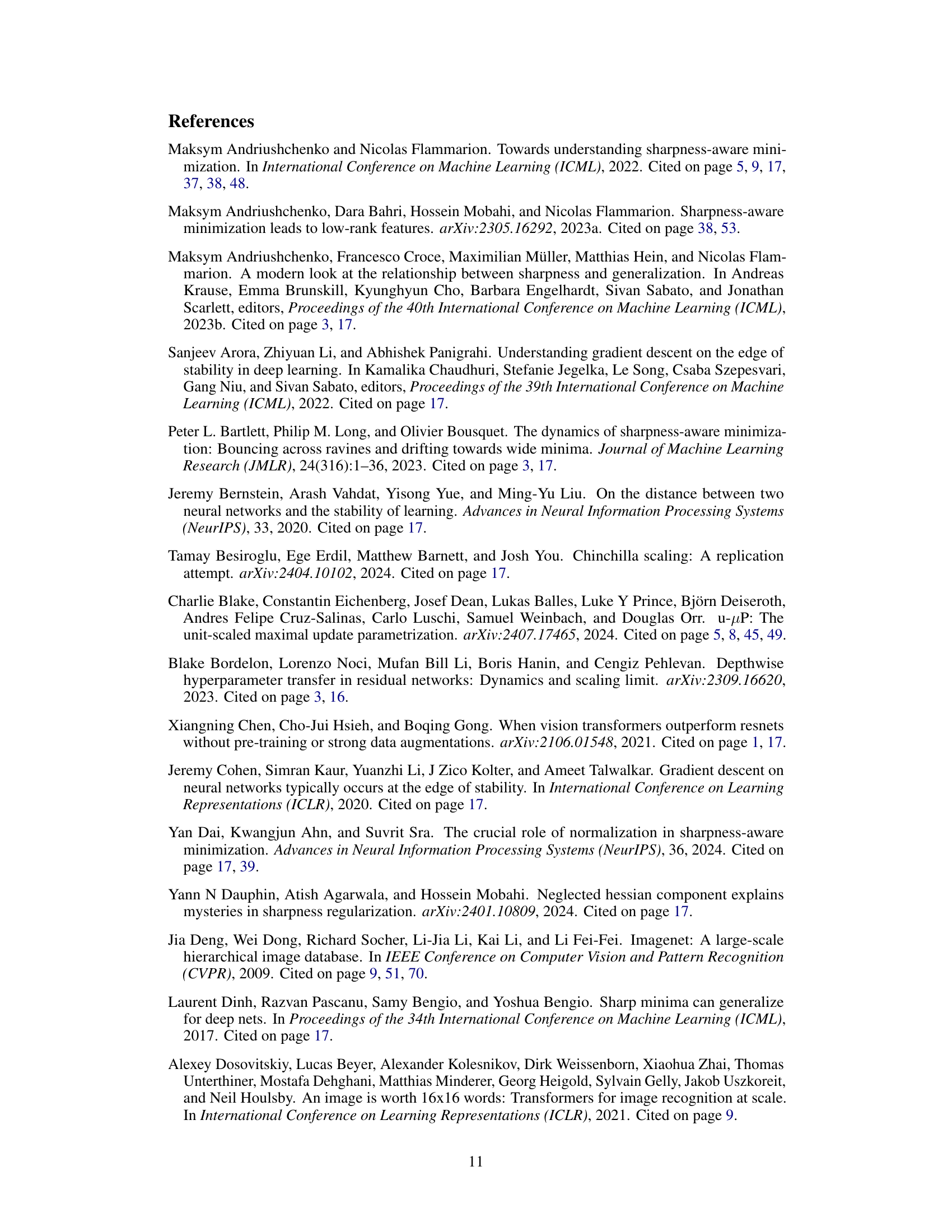
🔼 This table presents the average test accuracy and standard deviation obtained from four independent runs for ResNet-18 with a width multiplier of 4, trained on CIFAR10 using SGD as the base optimizer. It also shows the improvement in test accuracy achieved by SAM compared to using SGD alone. The results are shown for various SAM parameterizations (SP and µP²) and variants (SAM-ON, elementwise ASAM). This highlights the generalization performance of µP².
read the caption
Table 2: (Performance of µP²) Average test accuracy+standard deviation across 4 runs (+ improvement of SAM over SGD) for ResNet-18 with width multiplier 4 on CIFAR10 using SGD as a base optimizer.
🔼 This table summarizes the effects of layerwise perturbation scaling on the behavior of different SAM variants in the infinite-width limit. The left side shows that without layerwise scaling, different SAM variants perturb different subsets of layers. The right side shows that with the µP² parameterization, which incorporates layerwise perturbation scaling, all layers are effectively perturbed, enabling transfer of optimal hyperparameters (learning rate η and perturbation radius p) across different model widths.
read the caption
Table 1: (Layerwise perturbation scaling for effective perturbations in µP) Without layerwise perturbation scaling (left), each SAM variant perturbs a different subset of layers at large width n→∞, but we provide the unique layerwise perturbation rescaling µP² (right) that achieves effective perturbations in all layers. This parameterization transfers both the optimal η and p across widths.
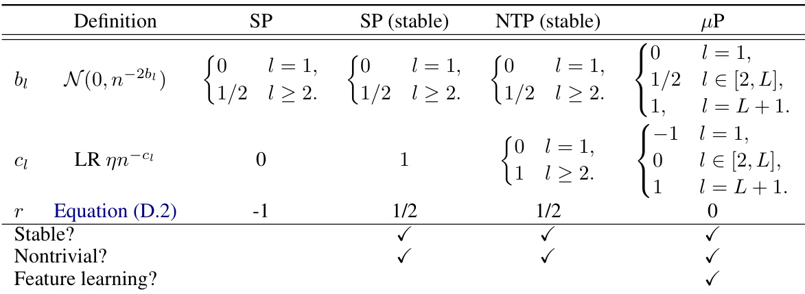
🔼 This table compares four different parameterizations of MLPs without biases: standard parameterization (SP), standard parameterization with maximal stable learning rate (SP (stable)), neural tangent parameterization (NTP), and maximal update parameterization (µP). For each parameterization, it shows the initialization of weights (bᵢ), the learning rate scaling (cᵢ), the maximal update scaling (r), whether the parameterization is stable, nontrivial, and whether it admits feature learning. The table provides a concise overview of various parameterization choices and their key characteristics, highlighting the differences in their ability to enable feature learning and stable training in the infinite-width limit.
read the caption
Table D.1: (bc-parametrizations) Overview over common implicitly used bc-parameterizations for training MLPs without biases in standard parametrization (SP), standard parametrization with maximal stable nonadaptive LR c = 1 (SP (stable)), neural tangent parametrization (NTP) and maximal update parametrization (µP).

🔼 The table shows four regimes for choosing perturbation scalings. Naive scaling is unstable and does not perturb any layers effectively. Global scaling (stable) is stable, but only perturbs the last layer. Effective scaling is stable and perturbs all layers effectively. The table provides a summary of different choices of layerwise perturbation scalings with their characteristics (stability, effective perturbations, etc.). It refers to a more detailed analysis in the appendix for further information.
read the caption
Table D.2: (Perturbation scalings) Overview over important choices of the global perturbation scaling pn−d and the layerwise perturbation scalings n−dι for training MLPs without biases with SAM: Naive scaling without width dependence (Naive), maximal stable global scaling along the original gradient direction (Global) and the unique scaling that achieves effective perturbations in all layers (Effective). An extensive overview that characterizes all possible choices of perturbation scaling is provided in Appendix F.1. Recall the gradient scaling c∇ := min(bL+1, cL+1).

🔼 This table shows the regimes of perturbation scaling for different choices of hyperparameters d and d₁, which control the stability and effectiveness of perturbations. The columns indicate whether effective perturbations are possible or if the gradient norm is dominated by each type of layer (input-like, hidden-like, output-like). Each row represents a range of values for hyperparameter d, and the checkmarks and crosses indicate which layer types can support effective perturbations within that range. For instance, when d = -1/2, effective perturbations are possible for all layer types, while when d > 1/2, only the output layer can have effective perturbations. The gradient norm constraint (D.1) is related to the scaling behavior and stability of the model.
read the caption
Table F.1: (Characterization of perturbation scalings) Overview over the regimes of all possible choices of d and d₁. A layer is effectively perturbed if and only if di satisfies (F.1). At least one layer must satisfy equality in its gradient norm constraint (D.1). This table summarizes which layers can exhibit effective perturbations, and which may dominate the gradient norm, given a choice of d. The choice d < -1/2 results in perturbation blowup r < 0. At the critical d = -1/2 (respectively, d = 0; d = 1/2) a input-like (respectively hidden-like; output-like) layer is effectively perturbed if and only if it dominates the gradient norm. Consequently d = -1/2 implies effective perturbations in at least one input-like layer.

🔼 This table shows the hyperparameter settings used for training ResNet-18 on CIFAR10 dataset using different optimization methods. It lists hyperparameters such as learning rate (LR), learning rate decay scheme, weight decay, momentum, label smoothing, perturbation radius (ρ), and output multiplier. The values for the standard parameterization (SP) are taken from a previous work by Müller et al. (2024). For the maximal update parameterization (µP), the base width is set to 0.5. The gradient norm scaling is adjusted according to the definition in the paper. The last layer is initialized to 0. The values for the perturbation radius (ρ) and learning rate (η) are tuned and reported in the paper.
read the caption
Table G.1: (ResNet-18 hyperparameters for CIFAR10) Hyperparameters for SP are taken from Müller et al. (2024). Learning rate and perturbation radius are tuned using the experiments in Appendix H.3.2. ResNets in µP have base width 0.5, gradient norm scaling according to Definition 4 and their last layer is initialized to 0.
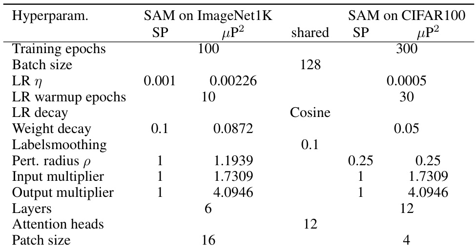
🔼 This table lists the hyperparameters used for training Vision Transformers (ViTs) with the standard parameterization (SP) and the proposed Maximal Update and Perturbation Parameterization (µP2). It shows hyperparameters for training on both ImageNet1K and CIFAR100 datasets. Note that the µP2 parameterization uses a base width of 384, initializes the last layer and query weights to 0, and scales the gradient norm contributions of all layers to 1. The hyperparameters for SP are taken from Müller et al. (2024), while those for µP2 were tuned using 3 independent runs of Nevergrad NGOpt.
read the caption
Table G.2: (Vision Transformer hyperparameters) Hyperparameters for SP are taken from Müller et al. (2024) using AdamW as a base optimizer. ViTs in µP have base width 384, last layer and query weights are initialized to 0 and gradient norm contributions of all layers are scaled to (1).

🔼 This table shows the training time per epoch for different model architectures and widths using SAM in the µP² parameterization. The architectures include ResNet-18 on CIFAR10 and Vision Transformers (ViTs) on CIFAR100 and ImageNet1K. The time per epoch is shown for various width multipliers (0.5, 1, 2, 4). This data provides insights into the computational cost of training these models with the proposed method.
read the caption
Table G.3: (Training time per epoch) Training time (in seconds) per epoch of the entire data loading and training pipeline of SAM in µP² on a single NVIDIA A10G GPU.
Full paper#
