TL;DR#
Time-series analysis often relies on ‘black-box’ models which lack interpretability, hindering understanding of their predictions. Existing interpretable methods like shapelets lack generalizability. Foundation models aim for unified time-series representation, but often fail to offer explanations. This creates a need for methods that offer both generalizability and interpretability.
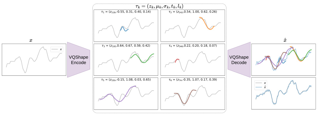
The paper introduces VQShape, a pre-trained model that uses vector quantization to represent time-series as abstracted shapes and associated attributes. This approach allows a unified representation across diverse domains. Experiments demonstrate VQShape achieves comparable performance to existing specialist models in classification tasks while also allowing for zero-shot learning and providing interpretable results. This work offers a significant contribution by successfully addressing the need for both interpretability and generalizability in time-series modeling.
Key Takeaways#
Why does it matter?#
This paper is important because it presents VQShape, a novel and effective approach to time-series representation learning. It addresses the limitations of existing black-box models by offering an interpretable and generalizable model. This opens avenues for zero-shot learning, improved understanding of time-series data across various domains, and enhances the development of more transparent and reliable machine learning models.
Visual Insights#
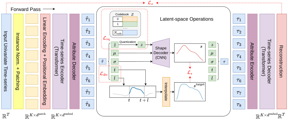
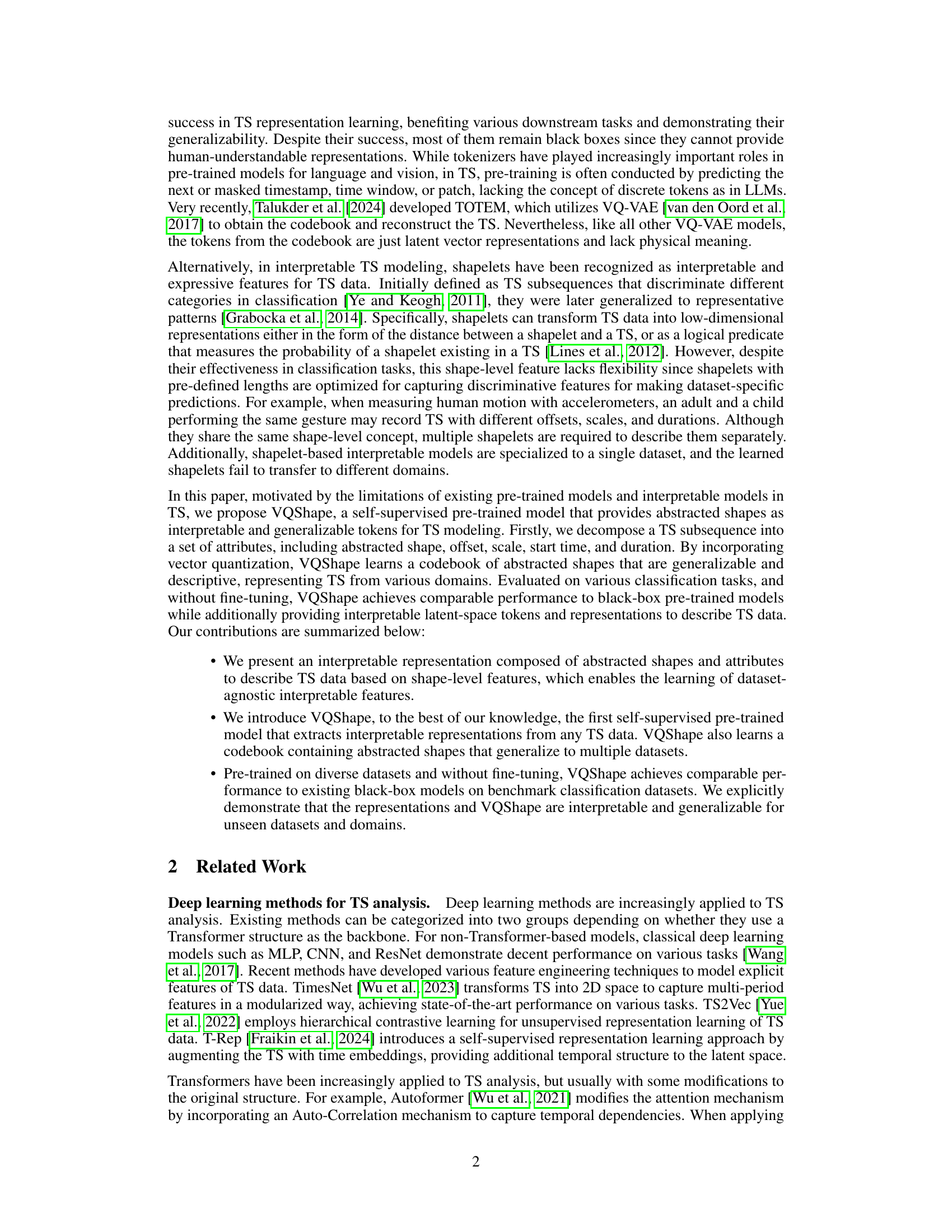
🔼 The figure shows an overview of the VQShape architecture. It is composed of a TS encoder, a TS decoder, a latent-space codebook, a shape decoder, and attribute encoders and decoders. The TS encoder takes a univariate time series as input and transforms it into patch embeddings using a transformer model. These embeddings are then passed through an attribute decoder that outputs a set of attribute tuples for each patch. These tuples are composed of the code for the abstracted shape of the patch, the offset, scale, start time, and duration. The attribute tuples are then quantized using vector quantization to select the nearest code in the codebook. The quantized codes are passed through a shape decoder to reconstruct the abstracted shapes of the patches. The abstracted shapes and attributes are then used to reconstruct the input time series. The figure also shows the pre-training objectives that are used to train the VQShape model.
read the caption
Figure 1: Overview of VQShape

🔼 This table presents a comparison of VQShape against several baseline methods for multivariate time series classification. The comparison includes classical methods, supervised learning methods, unsupervised representation learning methods, and pre-trained models. Performance is evaluated using mean accuracy and median accuracy, along with mean rank and median rank. The number of times each method achieved a top-1, top-3, win, or tie ranking are also shown, as well as the Wilcoxon p-value for the comparison. The statistics are presented both with and without considering results that were not available (N/A) for some baselines on certain datasets, providing a more complete comparison of performance.
read the caption
Table 1: Statistic and comparisons of the baselines and VQShape. The best case is marked with bold, the second best is marked with italic, and the third best is marked with underline. Some baselines fail are incompatible with some datasets which result in “N/A”. For fair comparison, we report the statistics with and without “N/A”. Complete results are presented in Table 5.
In-depth insights#
VQShape: A New Model#
VQShape presents a novel approach to time-series classification by leveraging vector quantization and interpretable shape representations. The model cleverly combines the power of transformer encoders for feature extraction with the interpretability of shapelets, creating a unified framework. A key innovation is its pre-trained codebook of abstracted shapes, which enables generalization across diverse datasets and domains, even achieving zero-shot learning capabilities. This generalizability is significant, moving beyond the limitations of many existing specialized TS models. Further, the interpretability offered through shape-level features facilitates a better understanding of the model’s decision-making process. However, the reliance on a fixed-length patch-based transformation introduces limitations, potentially hindering performance on irregularly sampled or very long time-series. Future work could explore dynamic patch sizes and alternative methods to enhance its adaptability to various TS characteristics.
Shape-Level Features#
The concept of “Shape-Level Features” in time-series analysis offers a powerful way to capture the underlying patterns and characteristics of data, moving beyond simple numerical representations. Shapelets, for example, are short, representative subsequences that can discriminate between different classes. However, traditional shapelet methods often suffer from limitations, such as being computationally expensive and struggling with variations in scale, offset, and duration. The use of vector quantization is particularly promising, allowing the encoding of time-series into a fixed set of “shape-tokens,” representing abstracted shapes. This approach enables generalizability across domains and datasets, creating a more unified representation space. Abstracted shapes as tokens represent a significant advancement, providing both interpretability and scalability. This approach enables the construction of interpretable classifiers which can generalize to previously unseen datasets and domains, a crucial step toward creating robust and trustworthy AI systems. The success of this method highlights the importance of moving away from black-box models, focusing instead on designs which provide both performance and the crucial advantage of human-interpretability.
Interpretable Tokens#
The concept of “Interpretable Tokens” in time-series analysis is crucial for bridging the gap between complex model outputs and human understanding. These tokens, unlike typical latent representations in black-box models, offer a meaningful interpretation of underlying time-series patterns. Ideally, they would be concise, easily visualized, and directly related to identifiable features within the time-series data, such as shapes or trends. The interpretability of these tokens enhances model transparency and trust, allowing for more effective debugging, analysis, and potential insights into the data itself. However, achieving truly interpretable tokens requires careful consideration of the tokenization process, which should strive for data-agnostic generalization to diverse time-series domains, and avoid domain-specific biases. The choice of feature representation that feeds into tokenization is vital for achieving meaningful interpretability. For example, using shape-level features that capture underlying patterns regardless of scale, or offset, is much more valuable than simpler representations based on raw data points. Developing methods for visualizing these tokens is crucial, providing a way to directly connect model representations to the temporal dynamics of the data. Methods such as visualization of the codebook might prove essential. Ultimately, the success of interpretable tokens hinges on the ability to strike a balance between the model’s ability to capture complex patterns and its capacity for producing easily interpretable outputs.
Generalizability Test#
A robust ‘Generalizability Test’ for a time-series model should go beyond simple in-domain validation. It needs to demonstrate the model’s ability to handle unseen data distributions, potentially spanning different domains or application areas. Key aspects would include evaluating performance on datasets with varying sampling rates, lengths, and noise levels; those with different characteristics from the training data. Furthermore, a rigorous test must consider transfer learning scenarios where the model, perhaps with minimal fine-tuning, is applied to a completely new task or domain. Quantifiable metrics, like classification accuracy and statistical significance tests, are essential. Zero-shot learning, a particularly stringent evaluation, assesses performance on previously unseen datasets without any adaptation, demonstrating true generalizability. Qualitative analysis, demonstrating the interpretability of model predictions across different domains is also important. A strong test should include a comparative analysis against other state-of-the-art models and classical approaches, highlighting VQShape’s advantages in terms of both performance and interpretability.
Future Directions#
Future research could explore several promising avenues. Extending VQShape’s capabilities to handle multivariate time series more effectively is crucial, potentially through advanced techniques that capture complex interdependencies between variables. Improving the efficiency of the pre-training process is another key area, perhaps by developing more sophisticated self-supervised learning objectives or leveraging transfer learning from other domains. Investigating the impact of different codebook sizes and dimensionality reduction methods on the interpretability and generalizability of VQShape’s representations warrants further investigation. Applying VQShape to various downstream tasks beyond classification, such as forecasting, anomaly detection, and imputation, would demonstrate its wider applicability. Finally, a deeper exploration of the learned shape representations and their connection to domain-specific knowledge could unlock valuable insights into the underlying patterns of time-series data across various applications. These advancements would enhance VQShape’s practicality and expand its impact in the field.
More visual insights#
More on figures

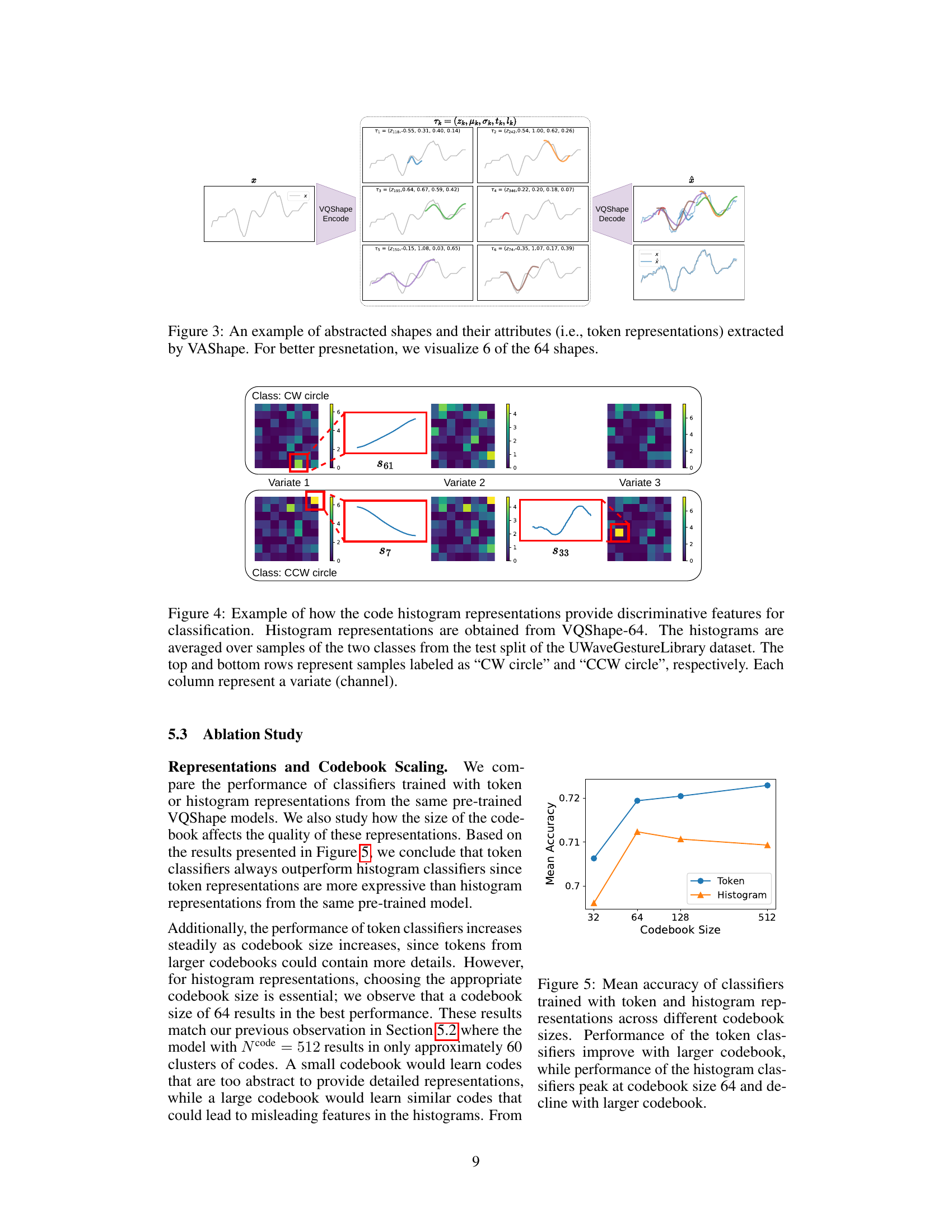
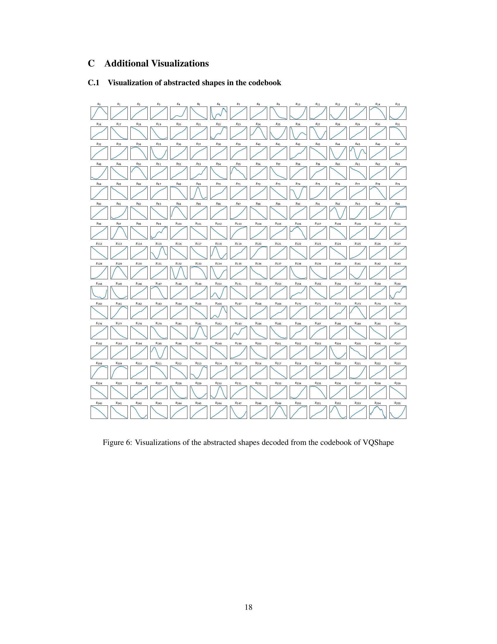
🔼 This figure visualizes the 512 abstracted shapes contained within the codebook of the VQShape model. Each shape is represented as a line graph, showing its unique form. The visualization helps demonstrate the diversity and variety of shapes learned by the model, and provides a visual representation of the model’s capacity to represent diverse time series data.
read the caption
Figure 6: Visualizations of the abstracted shapes decoded from the codebook of VQShape
🔼 This figure provides a detailed overview of the VQShape architecture. It illustrates the flow of data through the model, starting with the time-series input (x). The input undergoes a TS encoding process using a patch-based transformer encoder to produce latent embeddings. These embeddings are then passed through an attribute decoder, which extracts attributes such as abstracted shapes, offsets, scales, starting positions and durations. Vector quantization selects the closest code for each abstracted shape from a learned codebook. The resulting quantized attribute tuple is used to produce the final shape representations (sk) via shape decoding, and the reconstructed TS (x) via attribute encoding and reconstruction. The figure shows the various components and their interactions in the VQShape architecture.
read the caption
Figure 1: Overview of VQShape

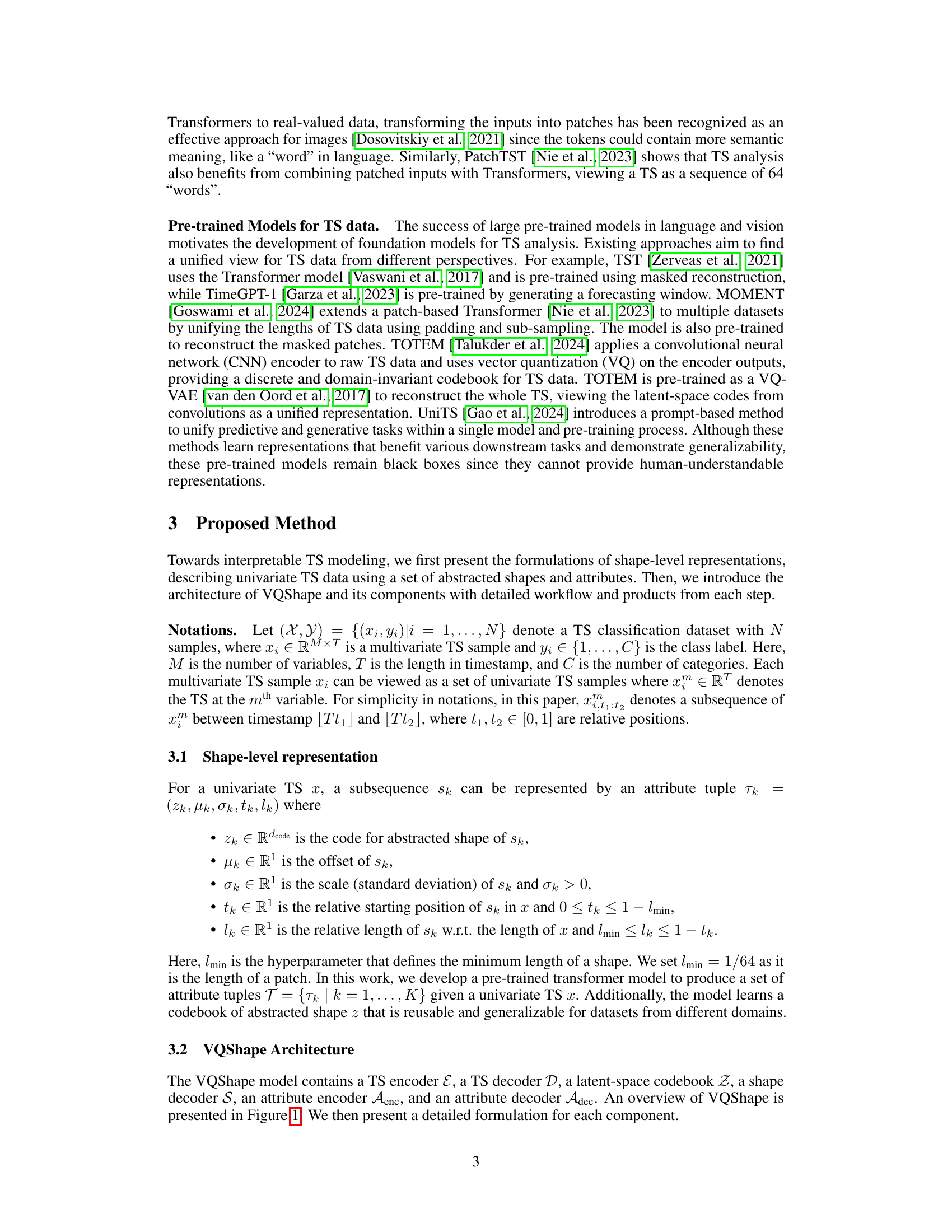
🔼 This figure demonstrates how the code histogram representations learned by VQShape-64 can distinguish between different classes in the UWaveGestureLibrary dataset. It shows the average code histograms for two classes (“CW circle” and “CCW circle”) across three different variates (channels). The significant differences in code frequencies between the two classes highlight the discriminative power of these representations for classification. Each histogram bar visually represents the frequency of a specific shape code, allowing for direct interpretation of the feature patterns that distinguish the two classes.
read the caption
Figure 4: Example of how the code histogram representations provide discriminative features for classification. Histogram representations are obtained from VQShape-64. The histograms are averaged over samples of the two classes from the test split of the UWaveGestureLibrary dataset. The top and bottom rows represent samples labeled as “CW circle” and “CCW circle”, respectively. Each column represent a variate (channel).
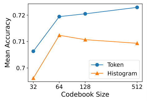
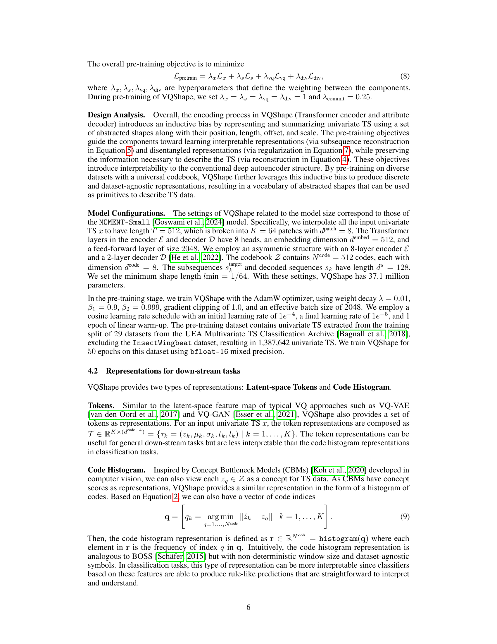
🔼 This figure shows the performance of classifiers trained using two different types of representations extracted from the VQShape model: token and histogram representations. The x-axis represents the codebook size used during training, while the y-axis shows the mean accuracy achieved on a classification task. The results indicate that token-based classifiers consistently improve in accuracy as the codebook size increases, suggesting that more detailed representations are beneficial. In contrast, histogram-based classifiers exhibit an optimal performance around a codebook size of 64, with accuracy declining as the codebook size increases beyond this point.
read the caption
Figure 5: Mean accuracy of classifiers trained with token and histogram representations across different codebook sizes. Performance of the token classifiers improve with larger codebook, while performance of the histogram classifiers peak at codebook size 64 and decline with larger codebook.

🔼 This figure shows the architecture of the VQShape model, which is composed of a TS encoder, a TS decoder, a latent-space codebook, a shape decoder, and an attribute encoder/decoder. The TS encoder transforms a univariate TS into patch embeddings that are fed into a transformer model to produce latent embeddings. The attribute decoder extracts attribute tuples (code for abstracted shape, offset, scale, start time, and duration) from the latent embeddings. Vector quantization selects discrete codes from the codebook based on Euclidean distance. The shape decoder takes the code and outputs a normalized subsequence with offset and scale removed. Finally, the attribute encoder and decoder reconstruct the attribute tuple and the whole TS.
read the caption
Figure 1: Overview of VQShape

🔼 This figure provides a detailed overview of the VQShape architecture. It shows the different components, including the TS encoder, the TS decoder, the latent-space codebook, the shape decoder, and the attribute encoder/decoder. The data flow is illustrated, showing how the model processes time-series data to extract interpretable representations.
read the caption
Figure 1: Overview of VQShape

🔼 This figure visualizes the distribution of 512 codes in the codebook of the VQShape model. The codes were reduced to two dimensions using t-SNE, a dimensionality reduction technique. The plot shows that the codes cluster into approximately 60 groups, suggesting that only around 60 distinct abstracted shapes are learned by the model, despite the larger codebook size. This indicates a degree of redundancy or similarity among the learned shapes.
read the caption
Figure 7: t-SNE plot of the codes.
🔼 This figure shows the architecture of the VQShape model, illustrating the flow of data through the different components. The time series (TS) is first encoded into patches using a transformer encoder, generating patch embeddings. These embeddings are then processed by the transformer model, resulting in latent embeddings. The attribute decoder extracts attributes like abstracted shape, offset, scale, start time, and duration from the latent embeddings. Vector quantization then maps these attributes to a discrete codebook of abstracted shapes. Finally, a shape decoder reconstructs the original TS subsequence using this codebook. The encoder and decoder, along with the codebook, form the core of VQShape’s learning process. The attribute encoder and decoder are critical for creating an interpretable representation that links the latent space to shape-level features.
read the caption
Figure 1: Overview of VQShape
More on tables

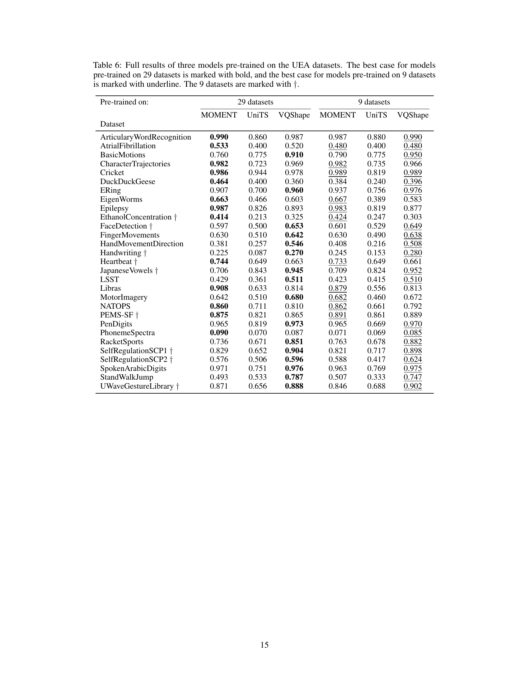
🔼 This table compares the performance of three pre-trained models (MOMENT, UniTS, and VQShape) on the UEA dataset. It shows the mean accuracy, median accuracy, mean rank, and number of times each model achieved the top-1 rank across 29 datasets. The results are separated into two groups: those pre-trained on all 29 datasets and those pre-trained on a smaller subset of 9 datasets. The best performance for each model and each dataset is bolded to highlight the best performing model in the comparison.
read the caption
Table 2: Comparison between three models pre-trained on all or a subset of the UEA datasets. The best cases are marked with bold. Complete results are presented in Table 6.
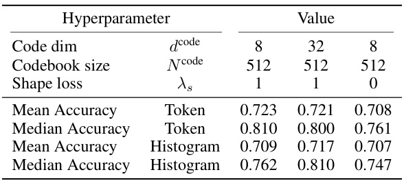
🔼 This ablation study explores the impact of varying the code dimension (dcode) and shape reconstruction loss (λs) on the performance of VQShape. Three configurations are compared: the default setting, a model with a reduced code dimension, and a model without shape loss. For each configuration, mean and median accuracy are reported for both token-based and histogram-based classifiers.
read the caption
Table 3: Statistics of ablation cases on code dimension and shape reconstruction loss.

🔼 This table compares the performance of VQShape against various baseline methods for multivariate time series classification. The baselines are categorized into classical methods, supervised learning methods, unsupervised representation learning methods, and pre-trained models. Performance is measured by mean accuracy, median accuracy, and mean rank across 29 datasets. The table notes that some baselines are incompatible with some datasets, resulting in missing values. To account for this, statistics are shown both with and without the missing values. The best performing model in each metric is highlighted.
read the caption
Table 1: Statistic and comparisons of the baselines and VQShape. The best case is marked with bold, the second best is marked with italic, and the third best is marked with underline. Some baselines fail are incompatible with some datasets which result in “N/A”. For fair comparison, we report the statistics with and without “N/A”. Complete results are presented in Table 5.

🔼 This table compares the performance of VQShape against various baseline methods for multivariate time series classification. The baselines are categorized into classical methods, supervised learning methods, unsupervised representation learning methods, and pre-trained models. Performance is measured by mean accuracy, median accuracy, and mean rank across 29 datasets. The table highlights the best, second best, and third best performing methods for each metric. Due to incompatibility issues with some datasets, results are presented both with and without the N/A values to provide a more complete comparison. Detailed results for each dataset are available in Table 5.
read the caption
Table 1: Statistic and comparisons of the baselines and VQShape. The best case is marked with bold, the second best is marked with italic, and the third best is marked with underline. Some baselines fail are incompatible with some datasets which result in “N/A”. For fair comparison, we report the statistics with and without “N/A”. Complete results are presented in Table 5.

🔼 This table presents a comparison of VQShape’s performance against various baseline methods for multivariate time series classification. The baselines are categorized into classical methods, supervised learning methods, unsupervised representation learning methods, and pre-trained models. The table shows the mean and median accuracy, mean and median rank, and number of times each method achieved top-1, top-3 ranks and win/tie results across the 29 datasets. Wilcoxon p-values indicate the statistical significance of the differences in performance between VQShape and other methods. The table also includes results both with and without considering datasets where some baselines failed (N/A). Complete results are in Table 5.
read the caption
Table 1: Statistic and comparisons of the baselines and VQShape. The best case is marked with bold, the second best is marked with italic, and the third best is marked with underline. Some baselines fail are incompatible with some datasets which result in “N/A”. For fair comparison, we report the statistics with and without “N/A”. Complete results are presented in Table 5.
🔼 This table compares the performance of VQShape against various baseline methods for multivariate time series classification tasks. It shows the mean and median accuracy, mean and median rank, number of times each method achieved top-1 and top-3 ranks, number of wins/ties/losses, and the Wilcoxon p-value. The comparison includes classical methods, supervised learning methods, unsupervised representation learning methods, and other pre-trained models. Results are shown with and without considering datasets where some methods failed, providing a more comprehensive comparison.
read the caption
Table 1: Statistic and comparisons of the baselines and VQShape. The best case is marked with bold, the second best is marked with italic, and the third best is marked with underline. Some baselines fail are incompatible with some datasets which result in “N/A”. For fair comparison, we report the statistics with and without “N/A”. Complete results are presented in Table 5.

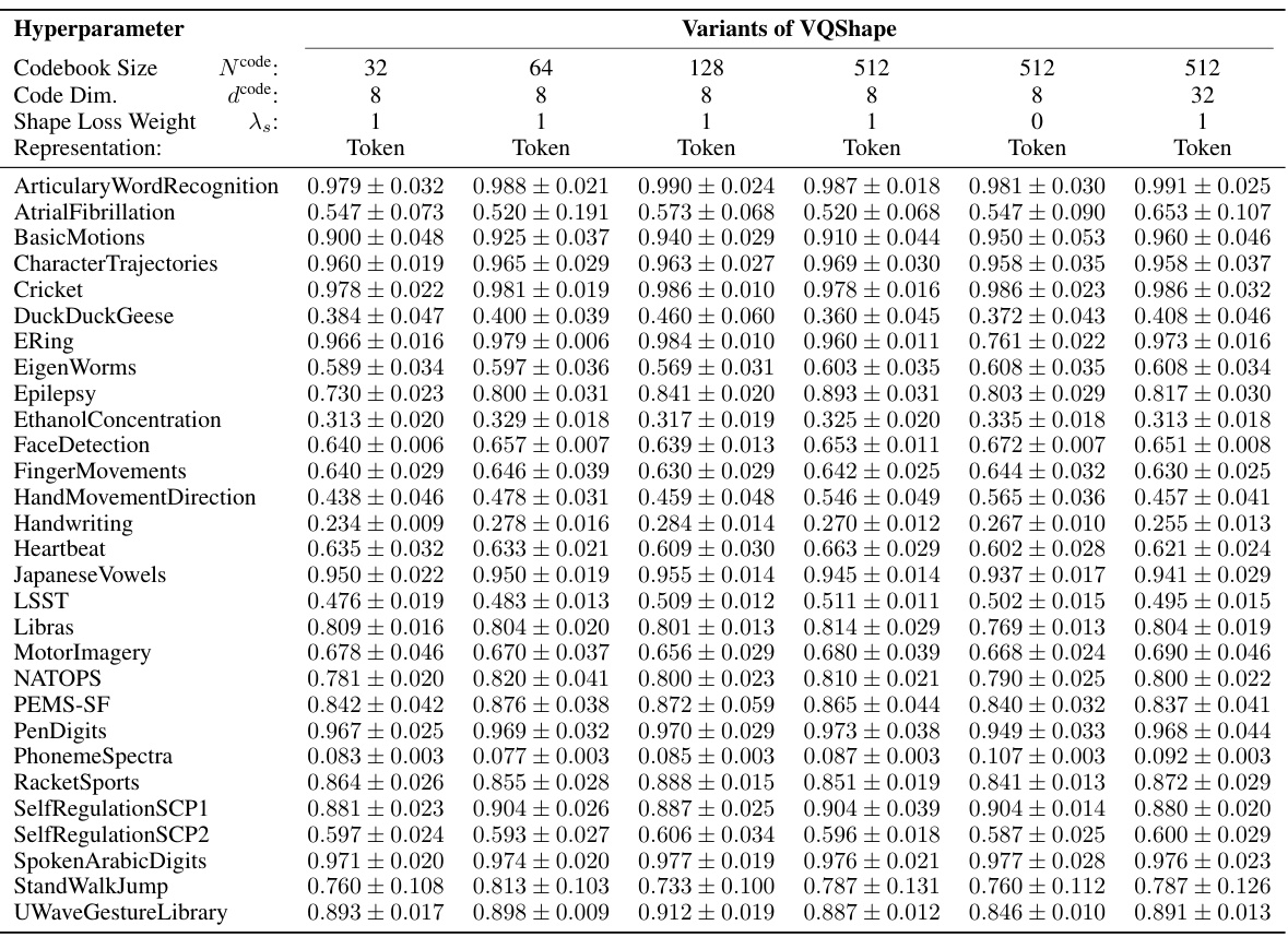
🔼 This table presents the classification accuracy results of various time series classification models on 29 benchmark datasets from the UEA archive. The models include classical methods (DTW, STRF), supervised learning models (DLinear, Autoformer, FEDformer, PatchTST, TimesNet), unsupervised representation learning models (TS-TCC, TST, T-Rep, TS2Vec), pre-trained models (MOMENT, UniTS), and the proposed VQShape model. The best, second best, and third-best performing models for each dataset are highlighted.
read the caption
Table 5: Full benchmark results on the 29 UEA datasets. For each dataset, the best case is marked with bold, the second best is marked with italic, and the third best is marked with underline.
Full paper#

