TL;DR#
Many real-world optimization problems involve parameters that are not fully known initially. Existing methods often assume all parameters are revealed simultaneously, which is unrealistic. This limitation significantly impacts the quality of solutions. This paper addresses this crucial issue.
The research proposes a novel framework called Multi-Stage Predict+Optimize, which models the sequential revelation of parameters. It introduces three training algorithms specifically designed for neural networks used in predicting parameters and solving Mixed Integer Linear Programs (MILPs). The algorithms are compared against existing approaches on three benchmarks, demonstrating improved learning performance.
Key Takeaways#
Why does it matter?#
This paper is crucial for researchers working on optimization problems with sequentially revealed parameters; it introduces a novel framework and efficient algorithms, advancing the state-of-the-art and opening new avenues for research in various applications such as scheduling and resource allocation.
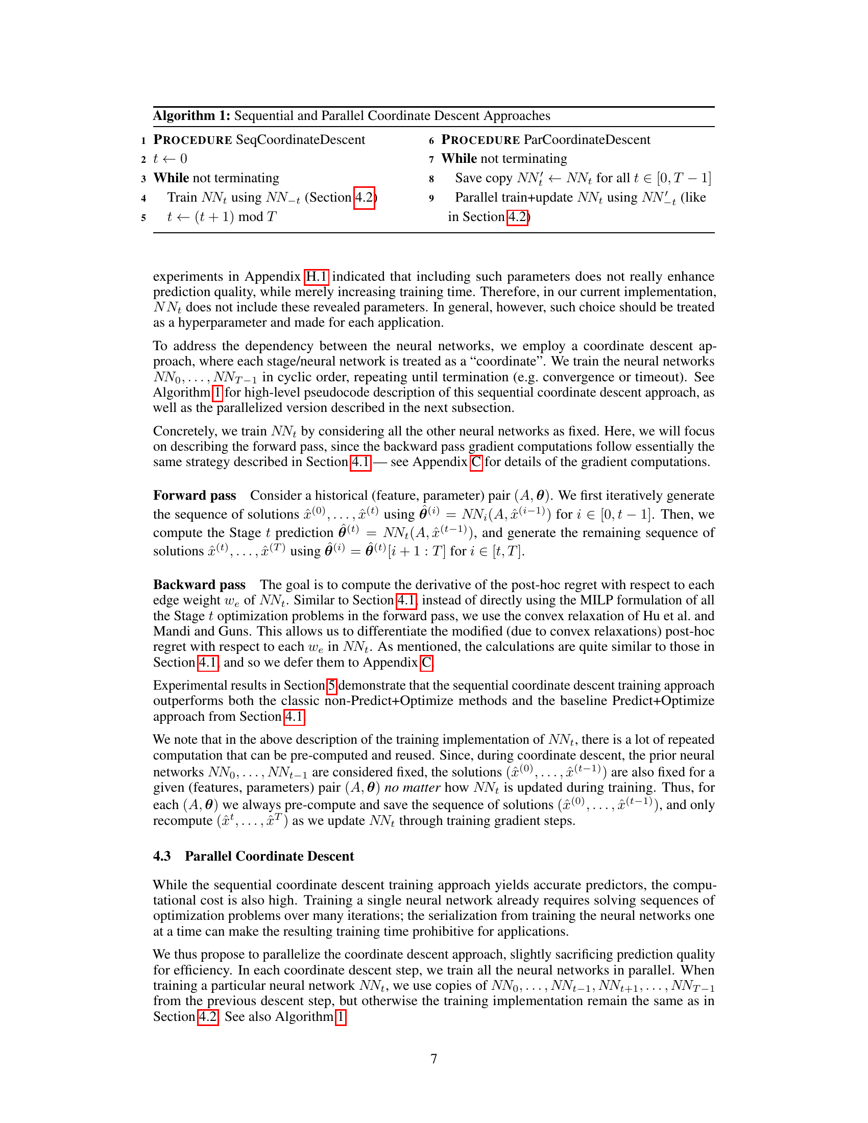
Visual Insights#
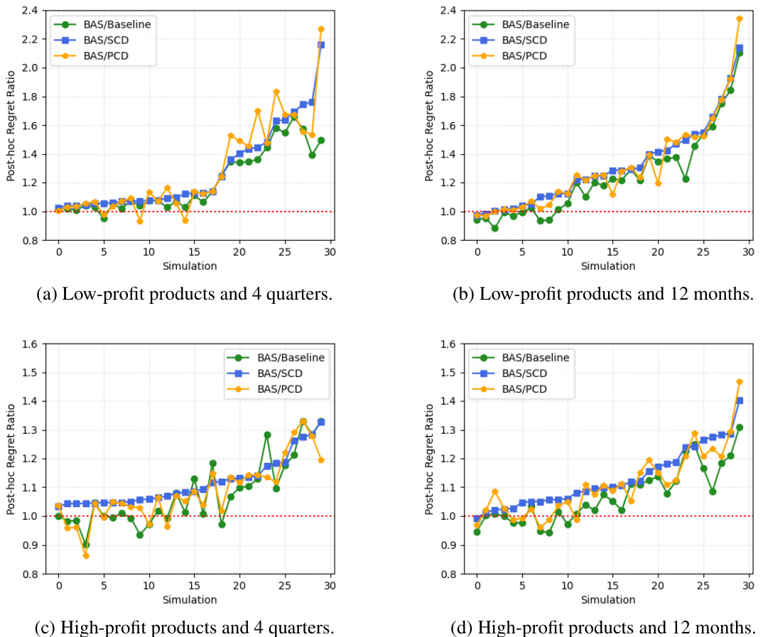
🔼 This figure presents a comparison of the performance of three different training methods (Baseline, SCD, and PCD) against a standard baseline method (BAS) for the production and sales problem. The x-axis represents the simulation number, and the y-axis shows the ratio of the post-hoc regret of BAS to the post-hoc regret achieved by each of the three methods. Points above the red dashed line (ratio = 1) indicate that a method outperforms BAS, while points below indicate that BAS performs better. Across all four scenarios (low-profit products with 4 quarters, low-profit products with 12 months, high-profit products with 4 quarters, and high-profit products with 12 months), SCD consistently outperforms BAS. PCD and Baseline also generally outperform BAS, but with less consistency than SCD. The results illustrate the advantage of the proposed training methods over the standard baseline.
read the caption
Figure 1: BAS/Baseline, BAS/SCD, and BAS/PCD for the production and sales problem.

🔼 This table presents the results of the production and sales problem experiment. It shows the mean and standard deviation of the post-hoc regret for four different scenarios: low-profit with 4 stages, low-profit with 12 stages, high-profit with 4 stages, and high-profit with 12 stages. The post-hoc regret is a measure of the difference between the actual objective function value obtained using the predicted parameters and the optimal objective function value that could be obtained if the true parameters were known in advance. The results are reported for three different methods (SCD, PCD, and Baseline), as well as a standard regression method (BAS). The true optimal value (TOV) is also provided for comparison.
read the caption
Table 1: Mean post-hoc regrets and standard deviations for the production and sales problem.
In-depth insights#
Multi-Stage PO#
Multi-Stage Predict+Optimize (PO) extends the standard PO framework by addressing scenarios where unknown parameters are revealed sequentially, rather than all at once. This is a significant advancement, making the framework applicable to a broader range of real-world problems that involve dynamic updates and decisions over time. The core idea is to make predictions about the unknown parameters at each stage, using a prediction model trained on historical data and potentially integrating the results of previous stages. These predictions then inform an optimization problem, whose solution provides hard commitments for the current stage, while influencing the predictions for future stages. This creates a dynamic interplay between prediction and optimization, leading to potentially more robust and adaptable solutions. The paper further introduces novel training algorithms that effectively handle the sequential nature of parameter revelation and the interdependencies between different stages, including sequential and parallel coordinate descent approaches. These algorithms address the complex optimization and prediction trade-offs involved, offering a practical and effective way to leverage the power of Multi-Stage PO in solving complex, real-world problems.
MILP Training#
Training mixed-integer linear programs (MILPs) within a machine learning framework presents unique challenges. The non-differentiability of MILP solutions introduces significant hurdles for standard gradient-based optimization. The paper likely explores methods to address this, potentially through relaxations of the MILP into a differentiable form or by using techniques that can handle non-differentiable loss functions. Approximation techniques might be considered, trading off solution accuracy for computational efficiency, possibly using surrogate models that capture the essence of the MILP behavior while allowing for gradient computation. The core of ‘MILP Training’ will likely involve carefully designed loss functions that consider the optimization problem’s structure, possibly incorporating regret minimization for robust performance. Furthermore, the training process itself may be tackled with specialized optimization methods beyond standard backpropagation, perhaps incorporating techniques like coordinate descent or other iterative approaches to handle the intricate dependencies between stages. The success of this approach hinges on the ability to effectively balance the need for accuracy in solving the MILP subproblems within the broader machine-learning context and the need for computational feasibility.
Sequential Training#
Sequential training, in the context of multi-stage prediction+optimization, presents a unique set of challenges and opportunities. The sequential nature of the process, where predictions are updated and optimization decisions made across multiple stages, demands careful consideration. A key advantage is the ability to leverage information revealed in earlier stages to refine subsequent predictions, leading to improved overall optimization performance. However, this interdependency between stages also introduces challenges in model training. A naive approach of training individual models independently ignores this intricate relationship and may lead to suboptimal results. Therefore, advanced techniques like coordinate descent are often necessary to handle the complex interplay between stages, iteratively updating predictions and optimizing decisions until convergence. Sequential training offers a compelling approach to multi-stage prediction+optimization, but the model training complexity should not be underestimated. The careful selection of appropriate training algorithms is crucial for balancing predictive power and computational efficiency.
Regret Minimization#
Regret minimization, in the context of machine learning for optimization problems, focuses on minimizing the difference between the objective function value achieved by the chosen solution and the optimal solution that could have been found if the true parameters were known in advance. This approach contrasts with classical methods that focus solely on minimizing prediction error of model parameters. The key insight is that a small parameter prediction error doesn’t guarantee a good solution to the optimization problem. Regret minimization directly incorporates the optimization problem’s structure into the learning process, leading to more robust and effective solutions, especially when dealing with uncertainty. Different variants of regret (e.g., post-hoc regret, dynamic regret) exist, reflecting the timing of parameter revelation and the possibility of recourse actions. The choice of regret measure significantly impacts the learned model’s performance, and algorithms for minimizing regret often involve intricate techniques such as differentiable convex approximations or specialized optimization methods to handle non-differentiable objective functions. The effectiveness of regret minimization relies heavily on the availability of training data that reflects the real-world distribution of parameters and features. This makes data quality and quantity crucial factors in the success of regret minimization approaches.
Future Work#
The “Future Work” section of a research paper on multi-stage predict+optimize for linear programs would naturally explore several avenues. Extending the framework to handle more complex problem structures beyond mixed-integer linear programs (MILPs) is crucial, potentially encompassing non-linear or stochastic constraints. Improving the efficiency of the training algorithms is another key area. The current methods, while showing promise, can be computationally expensive; research into faster training techniques, including more sophisticated parallelization or distributed algorithms, would be beneficial. Investigating the impact of different neural network architectures on predictive performance and computational cost warrants further investigation. Addressing the ‘curse of dimensionality’ in high-dimensional parameter spaces is also important, requiring exploring techniques like dimensionality reduction or feature engineering. Finally, applying the framework to a broader range of real-world applications would further validate its effectiveness and identify new challenges, leading to further refinements and extensions.
More visual insights#
More on tables

🔼 This table presents the mean and standard deviation of the post-hoc regrets for the production and sales problem. The results are broken down by price group (low-profit and high-profit) and stage number (4 and 12). It also includes the results for four different training algorithms (PCD, SCD, Baseline, and a standard regression model called BAS), along with the true optimal value (TOV). Post-hoc regret is a measure of how well the prediction method performs compared to having perfect knowledge of the parameters beforehand. Lower numbers indicate better performance.
read the caption
Table 1: Mean post-hoc regrets and standard deviations for the production and sales problem.

🔼 This table presents the mean and standard deviation of post-hoc regrets for different methods on the investment problem, specifically when the initial capital is set to 50. The methods include SCD, PCD, Baseline, and BAS (best among standard regression models). The results are broken down by the number of stages (4 or 12) and the transaction factor (0.01, 0.05, or 0.1). The true optimal values (TOV) are also provided for comparison.
read the caption
Table 2: Mean post-hoc regrets and standard deviations for the investment problem when capital=50.

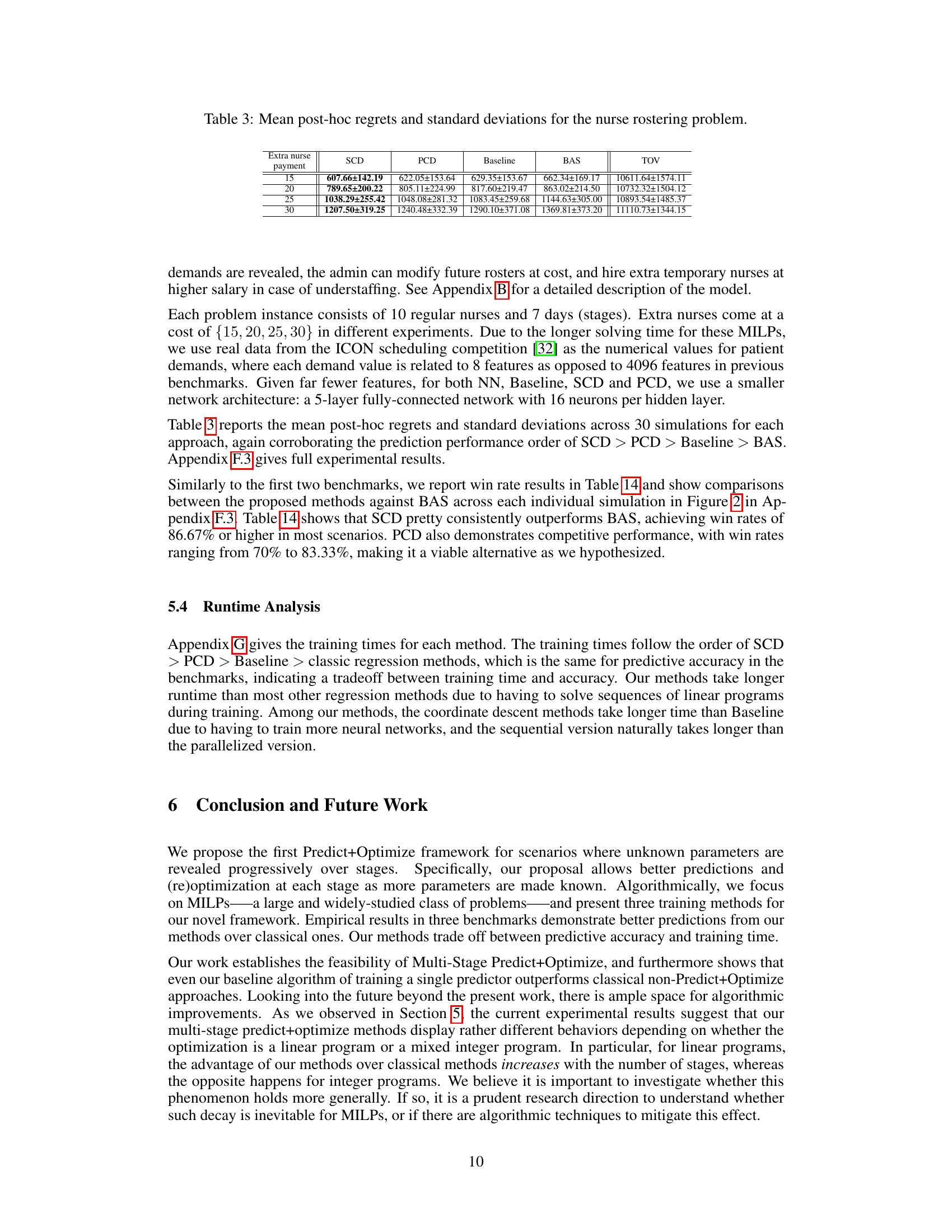
🔼 This table presents the mean and standard deviation of post-hoc regrets for four different methods (SCD, PCD, Baseline, and BAS) across 30 simulations in a nurse rostering problem. The results are broken down by four different levels of extra nurse payment (15, 20, 25, and 30). The TOV column shows the true optimal values (in hindsight) for comparison.
read the caption
Table 3: Mean post-hoc regrets and standard deviations for the nurse rostering problem.
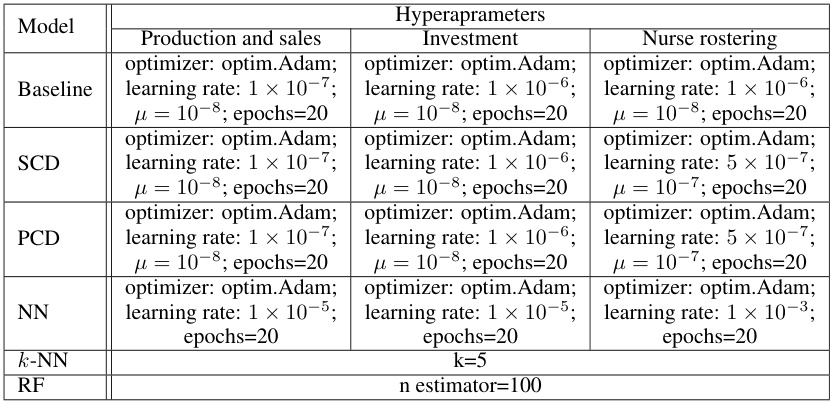
🔼 This table lists the hyperparameter settings used for each model (Baseline, SCD, PCD, NN, k-NN, RF) across three different optimization problems: Production and sales, Investment, and Nurse rostering. For each model and problem, the optimizer, learning rate, mu (log barrier regularization parameter), and number of epochs are specified. The table provides details on the parameter tuning process for each problem and algorithm.
read the caption
Table 4: Hyperparameters of the experiments on the three problems.
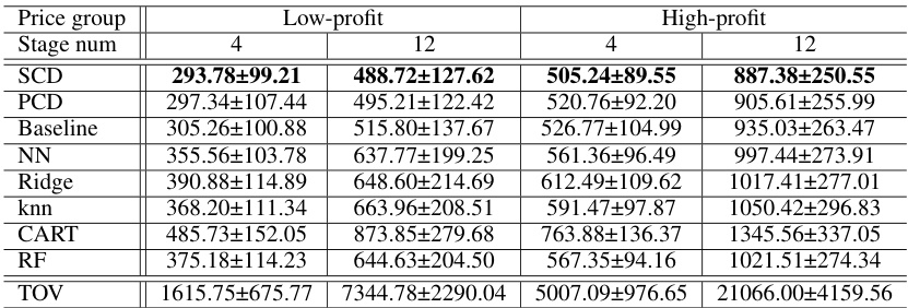
🔼 This table presents the mean and standard deviation of post-hoc regrets for different methods on the production and sales problem. The methods include three proposed training algorithms (Baseline, SCD, PCD) and several classical non-Predict+Optimize regression methods (NN, Ridge, k-NN, CART, RF). Results are shown for low-profit and high-profit price groups, with stage numbers (time horizons) of 4 and 12. The true optimal value (TOV) is also included for comparison.
read the caption
Table 1: Mean post-hoc regrets and standard deviations for the production and sales problem.

🔼 This table presents the percentage improvement of the proposed three training algorithms (Baseline, SCD, and PCD) compared to the standard regression models (BAS). It shows the improvement in post-hoc regret for different price groups (low-profit and high-profit) and numbers of stages (4 and 12). The table also provides a comparison between the three proposed methods, showing how much SCD and PCD improve over the baseline method.
read the caption
Table 6: Improvement ratios among Baseline, SCD, PCD, and standard regression models for the production and sales problem.

🔼 This table presents the win rates of Baseline, SCD, and PCD against BAS for the production and sales problem. The win rate indicates the percentage of simulations where a specific method outperformed BAS. This table shows that SCD consistently outperforms BAS across all scenarios, while PCD and Baseline also demonstrate advantages over BAS in most simulations, indicating their effectiveness in this problem. The win rates tend to improve with the increase of the number of stages.
read the caption
Table 7: Win rates for the production and sales problem.

🔼 This table presents the mean and standard deviation of post-hoc regrets for different methods (SCD, PCD, Baseline, NN, Ridge, k-NN, CART, RF) across 30 simulations of an investment problem with a capital of 25. The results are broken down by stage number (4 or 12) and transaction factor (0.01, 0.05, or 0.1). It allows comparison of the different methods’ performance in terms of minimizing post-hoc regret, a measure of how well the predictions from each model lead to good decisions when the actual parameters are revealed.
read the caption
Table 8: Mean post-hoc regrets and standard deviations of all methods for the investment problem when capital=25.

🔼 This table presents the mean and standard deviation of post-hoc regrets for different methods (SCD, PCD, Baseline, and BAS) across 30 simulations of the investment problem. The results are broken down by the transaction factor (0.01, 0.05, and 0.1) and the number of stages (4 and 12). The TOV column represents the true optimal values obtained using the true parameters.
read the caption
Table 2: Mean post-hoc regrets and standard deviations for the investment problem when capital=50.

🔼 This table presents the percentage improvements of the proposed three training algorithms (Baseline, SCD, PCD) over the standard regression methods (BAS) for the production and sales problem. The improvements are calculated as the percentage difference between the post-hoc regrets of the proposed methods and BAS. The table shows results for both low-profit and high-profit price groups, and for 4 and 12 stages. It helps illustrate how the relative performance of the algorithms changes with the number of stages and profit margin.
read the caption
Table 6: Improvement ratios among Baseline, SCD, PCD, and standard regression models for the production and sales problem.

🔼 This table presents the results of the production and sales problem experiment. It shows the mean and standard deviation of the post-hoc regret for different methods (Baseline, SCD, PCD, and standard regression methods) across 30 simulations. The results are broken down by price group (low-profit and high-profit) and the number of stages (T=4 and T=12). The post-hoc regret is a measure of how well the prediction models perform, considering both prediction error and optimization objective.
read the caption
Table 1: Mean post-hoc regrets and standard deviations for the production and sales problem.

🔼 This table presents the mean and standard deviation of post-hoc regrets for different methods (SCD, PCD, Baseline, NN, Ridge, k-NN, CART, RF) on the nurse rostering problem. The results are shown for various extra nurse payment levels (15, 20, 25, and 30), providing a comparison of the different methods’ performance under varying cost conditions. The ‘TOV’ column shows the true optimal values for each scenario. The table is used to assess the accuracy and robustness of different approaches to parameter prediction in the nurse rostering task.
read the caption
Table 3: Mean post-hoc regrets and standard deviations for the nurse rostering problem.

🔼 This table presents the percentage improvement of the three proposed training algorithms (Baseline, SCD, and PCD) over the standard regression models (BAS) for the production and sales problem. The improvements are calculated as the percentage difference in post-hoc regret between each proposed method and BAS. The table is broken down by price group (low-profit and high-profit) and the number of stages (4 and 12). It shows that the advantage of the proposed methods over BAS increases with the number of stages.
read the caption
Table 6: Improvement ratios among Baseline, SCD, PCD, and standard regression models for the production and sales problem.

🔼 This table presents the mean and standard deviation of post-hoc regrets for different models (Baseline, SCD, PCD, and standard regression models) on the production and sales problem. The results are broken down by price group (low-profit and high-profit) and the number of stages (4 or 12). The true optimal values are also provided for reference.
read the caption
Table 1: Mean post-hoc regrets and standard deviations for the production and sales problem.

🔼 This table presents the results of the production and sales problem experiment. It shows the mean and standard deviation of the post-hoc regret for four different scenarios: low-profit with 4 stages, low-profit with 12 stages, high-profit with 4 stages, and high-profit with 12 stages. The post-hoc regret is a metric that measures the difference between the objective function value obtained with the predicted parameters and the true optimal objective function value. The results are compared across different methods: PCD, SCD, Baseline, NN, Ridge, k-NN, CART, and RF. The TOV column displays the average true optimal objective function values across simulations.
read the caption
Table 1: Mean post-hoc regrets and standard deviations for the production and sales problem.

🔼 This table presents the mean post-hoc regrets and standard deviations for five different training methods applied to the production and sales problem. The methods include: training SCD with revealed parameters, training PCD with revealed parameters, SCD, PCD, and Baseline. The results are broken down by price group (low-profit and high-profit) and stage number (4 and 12). The table allows comparison of the impact of including revealed parameters in the training process and the relative performance of the different training approaches.
read the caption
Table 16: Mean post-hoc regrets and standard deviations of training SCD with revealed parameters, training PCD with revealed parameters, SCD, PCD, and Baseline for the production and sales problem.

🔼 This table presents the mean post-hoc regrets and standard deviations obtained using four different training methods for the production and sales problem. The methods compared are a simultaneous training method, Sequential Coordinate Descent (SCD), Parallel Coordinate Descent (PCD), and a baseline method. The results are broken down by price group (low-profit and high-profit) and stage number (4 and 12). The post-hoc regret is a measure of the effectiveness of a prediction model in the context of optimization problems. Lower values indicate better performance.
read the caption
Table 17: Mean post-hoc regrets and standard deviations of a simultaneous training method, SCD, PCD, and Baseline for the production and sales problem.
Full paper#
