↗ OpenReview ↗ NeurIPS Homepage ↗ Chat
TL;DR#
Generative models struggle with non-Euclidean data (e.g., spherical data, rotation matrices). Existing methods often rely on computationally intensive differential equation solvers for sampling, hindering their practical application. This limits the use of generative models in many fields where data naturally resides in non-Euclidean spaces.
This work introduces Manifold Free-Form Flows (M-FFF), a novel generative model that overcomes these limitations. M-FFF leverages a single feed-forward neural network for sampling and density estimation, bypassing the need to solve differential equations. This results in a method that is orders of magnitude faster than existing techniques, while achieving comparable or even better accuracy on various benchmarks. The generalizability of the M-FFF framework makes it suitable for a wide variety of Riemannian manifolds.
Key Takeaways#
Why does it matter?#
This paper is significant for researchers in machine learning and related fields because it introduces a novel and efficient approach to generate data on manifolds. It addresses the computational limitations of existing methods, making high-quality generative models feasible for various applications. The improved speed and performance open new avenues for using manifold-based generative models in diverse applications such as robotics, computer vision, and scientific data analysis. The approach is applicable to any Riemannian manifold with a known embedding and projection, expanding the range of problems that can be tackled by generative models.
Visual Insights#

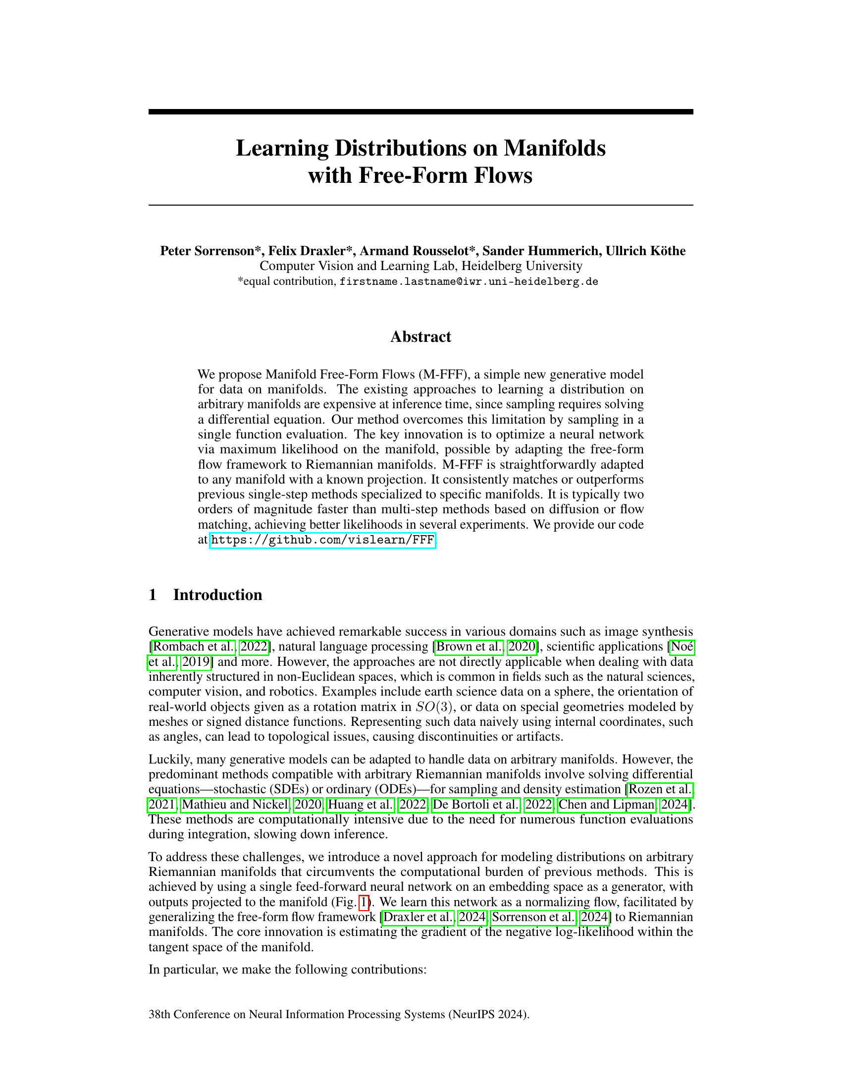
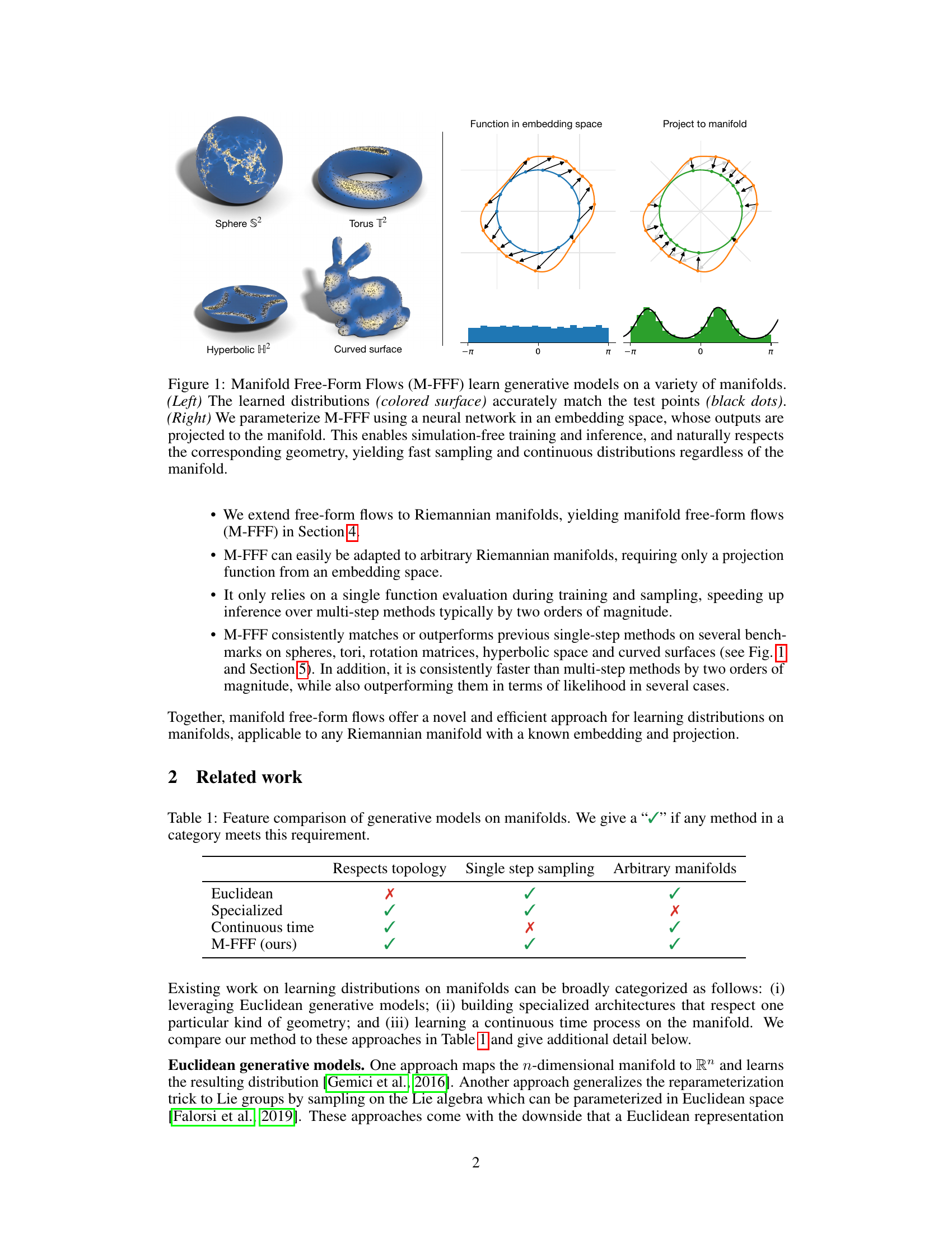
This figure shows examples of manifold free-form flows (M-FFF) applied to various manifolds. The left side shows the learned distributions (colored surfaces) which accurately match the given test points (black dots) on spheres, tori, hyperbolic surfaces, and curved surfaces. The right side illustrates the process of M-FFF. It uses a neural network to generate outputs in an embedding space. These outputs are then projected to the manifold, ensuring that the generated samples respect the underlying geometry. This approach allows for efficient and simulation-free training and inference, resulting in fast sampling and continuous distributions.

This table compares different generative models on manifolds based on three features: whether they respect the topology of the manifold, whether they allow for single-step sampling, and whether they are applicable to arbitrary manifolds. The table highlights the advantages of Manifold Free-Form Flows (M-FFF) by showing that it is the only method that satisfies all three criteria.
In-depth insights#
Manifold Flows#
Manifold flows represent a significant advancement in generative modeling, extending the capabilities of traditional normalizing flows to handle data residing on non-Euclidean manifolds. This is crucial because many real-world datasets, such as those encountered in robotics, computer vision, and scientific applications, exhibit inherent non-Euclidean structures. Unlike traditional flows operating in flat Euclidean space, manifold flows are designed to respect the underlying geometry and topology of the data manifold. This involves defining transformations that are consistent with the manifold’s structure, ensuring that generated samples remain within the manifold’s boundaries and that the probability density estimation accurately reflects the manifold’s curvature. A key challenge is efficiently computing the change of variables Jacobian as required for density estimation, often involving computationally expensive procedures like solving differential equations. Addressing this computational burden is a primary focus in the development of efficient manifold flow methods. Furthermore, generalizing manifold flow methods to arbitrary manifolds is an area of active research; ideally, a unified framework should enable seamless adaptation to various manifolds without requiring manifold-specific designs.
M-FFF: A New Model#
The proposed Manifold Free-Form Flows (M-FFF) model presents a novel approach to generative modeling on manifolds, addressing limitations of existing methods. Its key innovation is sampling in a single function evaluation, overcoming the computational burden of multi-step approaches requiring differential equation solving. M-FFF’s adaptability to various Riemannian manifolds is a significant strength, requiring only a known projection function. The model consistently outperforms or matches previous single-step methods across multiple benchmark datasets, while achieving significantly faster inference times. This efficiency is attributed to the clever optimization strategy, leveraging the free-form flow framework adapted to Riemannian manifolds. However, approximations are made, particularly concerning the Jacobian inverse, which could affect performance in complex scenarios. Despite these approximations, the model demonstrates robust performance, suggesting it offers a promising direction for generative modeling in non-Euclidean spaces.
Empirical Results#
An effective ‘Empirical Results’ section would meticulously detail experimental setup, datasets used, and evaluation metrics. Clear visualizations of key findings, such as plots comparing the proposed method against baselines, are crucial. The discussion should go beyond simple performance metrics; it needs to interpret the results in the context of the research questions, pointing out successes, failures, and unexpected behavior. A strong section would also address limitations of the experiments, acknowledging factors that might have affected the results and suggesting future work. Statistical significance, error bars, or confidence intervals must be rigorously reported to ensure the robustness of the claims. Finally, a comparative analysis of performance across different datasets or scenarios helps highlight the generalizability and limitations of the approach.
Limitations & Future#
The section titled “Limitations & Future” would critically analyze shortcomings of the proposed method, such as approximations in gradient estimation impacting accuracy, and computational efficiency relative to multi-step methods. Future work could explore refining the gradient estimator for improved accuracy and exploring applications beyond the tested manifolds. Addressing the scalability to higher dimensional manifolds and handling of non-isometric embeddings more robustly is key. Finally, comparative analyses against more diverse and complex real-world datasets would strengthen the method’s generalizability and utility. A thorough investigation into these aspects would provide a complete picture of the strengths and weaknesses of the approach, paving the way for valuable future enhancements and broader applicability.
Experimental Setup#
A robust experimental setup is crucial for validating the claims of a research paper. For a study on manifold free-form flows, the setup should detail the datasets used, emphasizing their characteristics (dimensionality, topology, size). Clearly describing data preprocessing steps (e.g., normalization, handling of missing values) is essential for reproducibility. The choice of evaluation metrics (e.g., negative log-likelihood, Wasserstein distance) and the rationale behind their selection need to be justified. Comparison with established baselines is vital, ensuring fair comparisons by using the same metrics and datasets. The experimental setup should also describe the models’ architectures (e.g., encoder, decoder structure), training hyperparameters (learning rate, batch size, optimizer), and the training process itself (e.g., number of epochs, early stopping criteria). Computational resources used (hardware, software, runtime) need to be specified for reproducibility. A rigorous experimental setup provides transparency and confidence in the reported results, enabling other researchers to validate and extend the work.
More visual insights#
More on figures
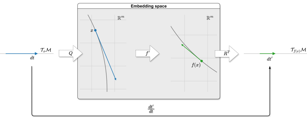
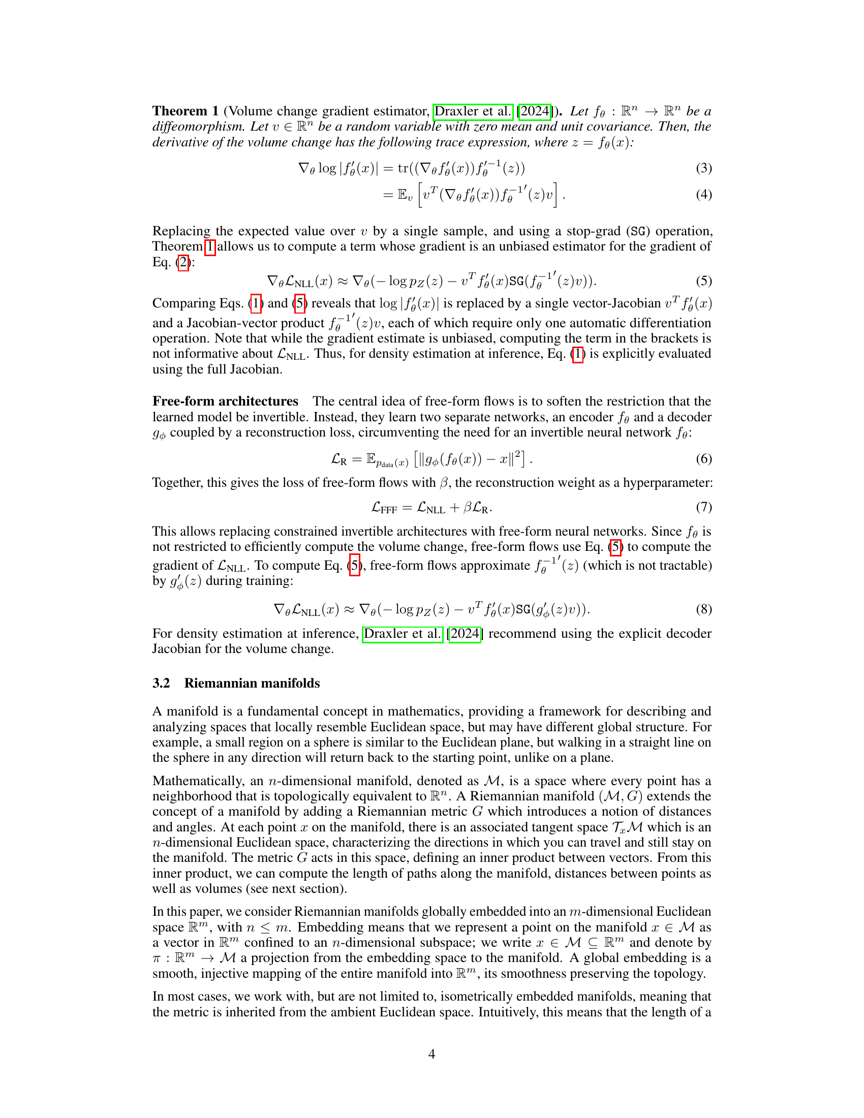
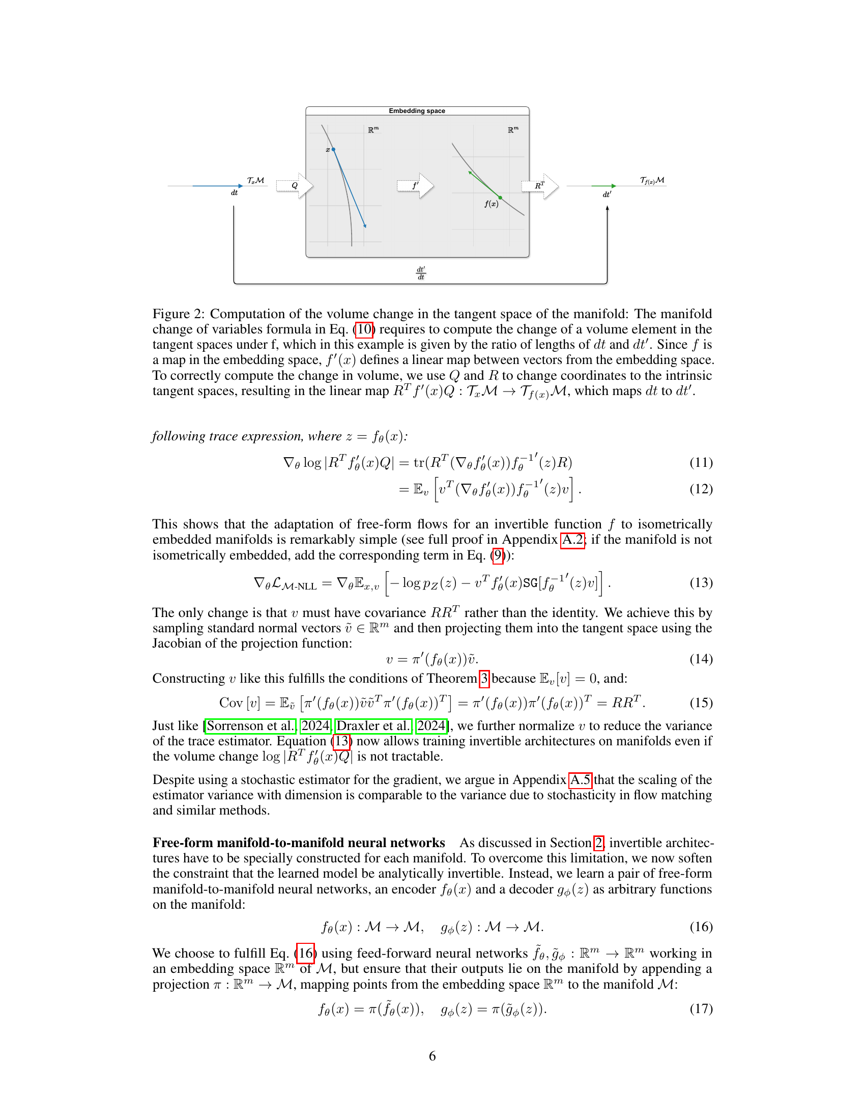
The figure shows how the volume change is computed in the tangent space of a Riemannian manifold. It illustrates that the Jacobian of a function acting on a manifold needs to be projected to the tangent space in order to correctly calculate the volume change. The projection is performed using orthonormal basis Q and R for the tangent spaces at x and f(x) respectively. This is because the function is defined on the embedding space, but volume change must be measured intrinsically on the manifold.

This figure shows examples of Manifold Free-Form Flows (M-FFF) applied to various manifolds. The left side illustrates how the learned probability distribution (shown as a colored surface) accurately represents the data points (black dots) on different manifolds such as a sphere, torus, and hyperbolic surface. The right side illustrates the M-FFF model architecture. It shows that the model uses a neural network to parameterize the distribution in an embedding space and then projects these parameters to the target manifold. This allows M-FFF to learn distributions on arbitrary manifolds efficiently.

This figure shows the log density plots generated by the Manifold Free-Form Flows (M-FFF) models for four different protein datasets (General, Glycine, Proline, and Pre-Proline). Each plot displays the log density as a function of two dihedral angles, Φ and Ψ, which are commonly used to represent the backbone conformation of proteins. The black dots represent the actual data points from the test dataset. The color scheme represents the density, where darker colors indicate lower density and lighter colors indicate higher density. The plots demonstrate that the M-FFF model accurately captures the distribution of the data points and satisfies the periodic boundary conditions of the dihedral angles.

This figure shows examples of Manifold Free-Form Flows (M-FFF) applied to various manifolds. The left side shows the learned probability distributions (colored surfaces) overlayed on point clouds of the test data. The right side illustrates the architecture, showing how a neural network in an embedding space generates samples that are then projected onto the manifold, demonstrating the model’s ability to generate data respecting the manifold’s geometry, offering a simulation-free method that is both fast and accurate.
More on tables

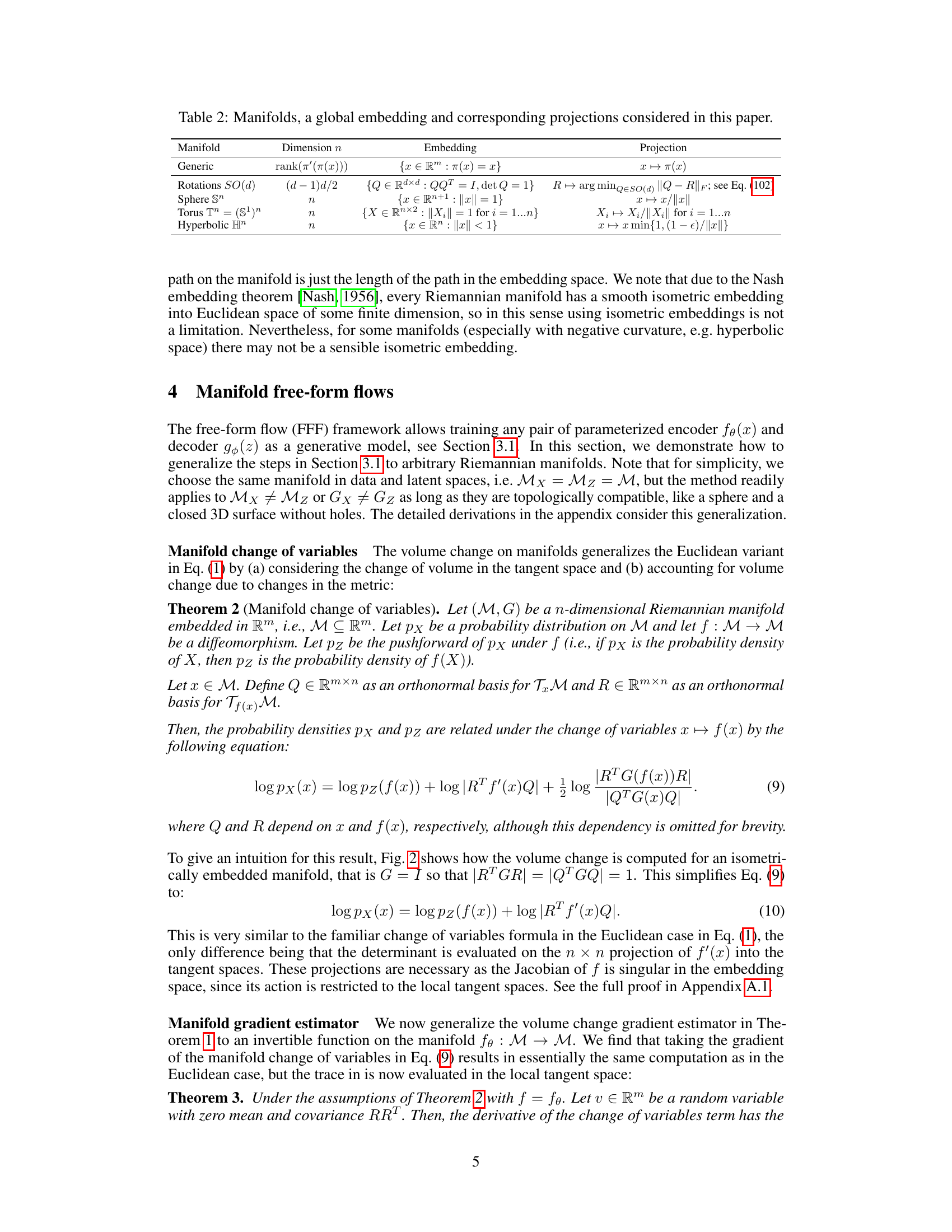
This table lists manifolds used in the paper, their dimensions, their embedding in Euclidean space, and the projection function used to project points from the embedding space onto the manifold. The embedding and projection are crucial for the method because the model operates in the embedding space and the gradient calculations are performed in the tangent space of the manifold. The table shows the specific mathematical forms for several common manifolds, providing concrete examples for the general framework.

This table compares the performance of Manifold Free-Form Flows (M-FFF) against other methods (both single-step and multi-step) for learning distributions on the special orthogonal group SO(3). The comparison is done using the test negative log-likelihood (NLL), a lower NLL indicating better performance. The results show that M-FFF consistently outperforms a specialized normalizing flow method and often outperforms multi-step methods, particularly when dealing with a higher number of mixture components in the synthetic data.

This table compares the performance of Manifold Free-Form Flows (M-FFF) against several other generative models on real-world datasets representing data points on a sphere (S2). The datasets are related to Earth science phenomena, such as volcanic eruptions, earthquakes, floods, and wildfires. The table shows the negative log-likelihood (NLL) achieved by each method. Lower NLL indicates better performance. The ‘Fast inference?’ column indicates whether the method is computationally efficient at inference time. The results indicate that M-FFF either matches or outperforms other single-step methods and often outperforms multi-step methods in terms of NLL, while also being significantly faster.

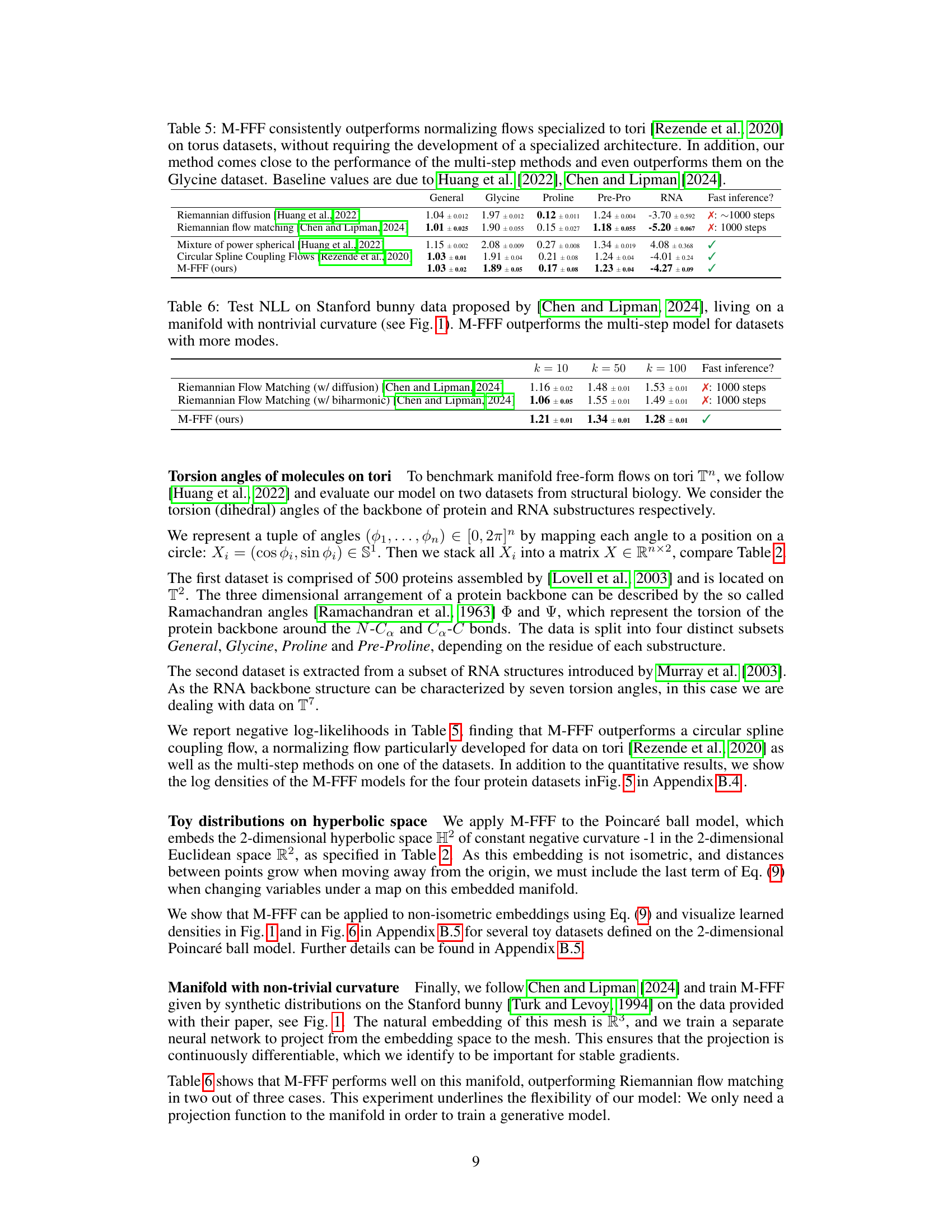
This table compares the performance of Manifold Free-Form Flows (M-FFF) against other methods for learning distributions on tori. It shows negative log-likelihood (NLL) scores for several datasets, demonstrating that M-FFF either matches or outperforms the previous state-of-the-art single-step and multi-step methods, especially on the Glycine dataset.

This table compares the performance of M-FFF against Riemannian Flow Matching models (with diffusion and biharmonic) on a Stanford bunny dataset. The dataset represents a manifold with non-trivial curvature. The results show negative log-likelihood (NLL) values for different numbers of modes (k) in the dataset. M-FFF achieves comparable or better performance than the multi-step methods, particularly for datasets with more modes.
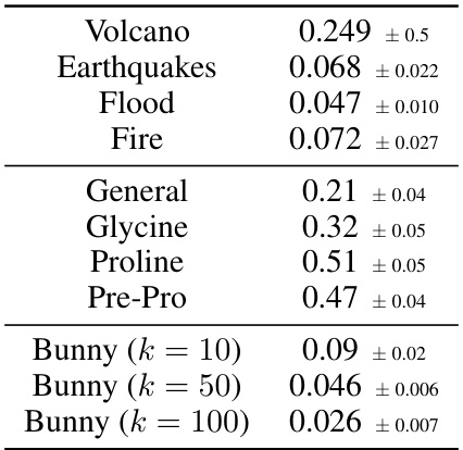
This table presents the Wasserstein-2 distances, a metric measuring the distance between two probability distributions, for various 2-dimensional manifolds. The manifolds include real-world geographical data (Volcano, Earthquakes, Flood, Fire) and data from structural biology (General, Glycine, Proline, Pre-Pro). Results are also given for the Stanford Bunny dataset, at different numbers of modes (k=10, k=50, k=100). The values represent the average Wasserstein-2 distance and its standard deviation, calculated from multiple experimental runs.
This table compares the performance of Manifold Free-Form Flows (M-FFF) against other methods (both single-step and multi-step) for learning distributions on the special orthogonal group SO(3). The comparison focuses on negative log-likelihood (NLL), a measure of how well the model fits the data. The results show that M-FFF consistently outperforms a specialized normalizing flow method and often outperforms multi-step approaches, especially as the number of mixture components in the data increases. The table also highlights the computational efficiency of M-FFF compared to multi-step methods which require many function evaluations.

This table compares the performance of M-FFF against other generative models on four real-world datasets representing earth science data on a sphere. The models are evaluated based on their negative log-likelihood (NLL), a metric where lower values indicate better performance. M-FFF is shown to outperform a previous single-step method, and shows mixed results compared to multi-step methods, potentially because the multi-step methods are better suited to data with large empty regions between data clusters.

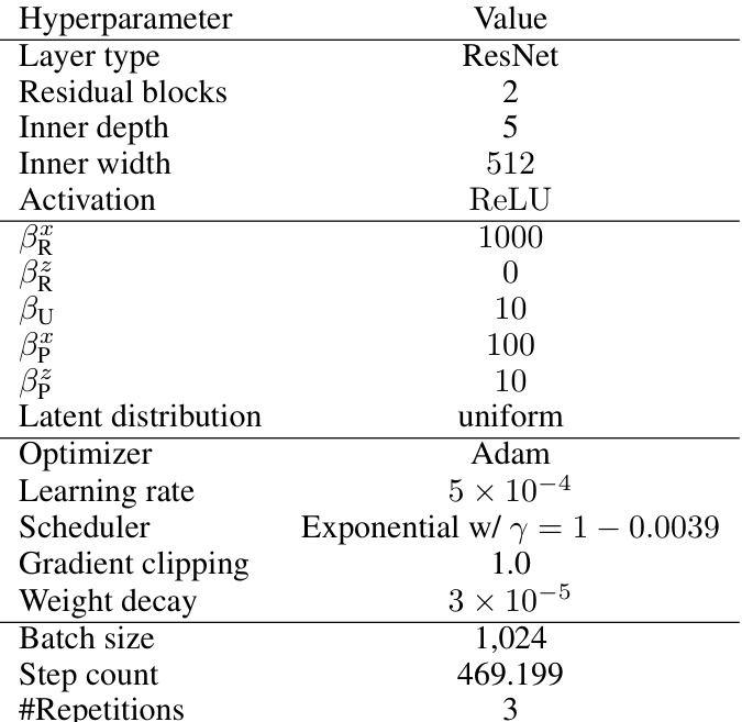
This table lists the hyperparameter values used for the earth data experiments in the paper. It includes choices for network architecture (layer type, residual blocks, inner depth, inner width, activation function), regularization parameters (βR, βU, βP), latent distribution, optimizer, learning rate, scheduler, gradient clipping, weight decay, batch size, step count, and number of repetitions. Note that βu and βp (regularization parameters) had the same values for both sample and latent spaces.

This table presents details about the datasets used in the experiments on the torus manifolds. It shows the number of instances (data points) in each dataset, and the amount of Gaussian noise added to the data during training to prevent overfitting. The datasets are split into training, validation, and test sets (80%, 10%, 10%, respectively).

This table compares different generative models on manifolds based on three key features: whether they respect the topology of the manifold, if they perform single-step sampling, and if they can handle arbitrary manifolds. The table shows that the proposed method (M-FFF) is unique in satisfying all three criteria, unlike existing approaches which may only meet one or two.

This table compares different generative models based on their ability to respect the topology of the manifold, whether they perform single-step sampling, and their applicability to arbitrary manifolds. It highlights the advantages of the proposed Manifold Free-Form Flows (M-FFF) method by showing that it satisfies all three criteria, unlike other existing methods.
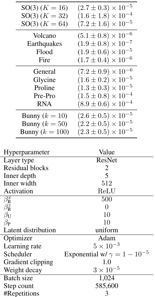
This table displays the reconstruction loss for each experiment performed in the paper. The reconstruction loss measures how close the model’s generated points are to the original data points. Low reconstruction loss indicates that the model accurately reconstructs the data and thus, supports the use of negative log-likelihoods (NLL) for model evaluation.
Full paper#
