Tighter Convergence Bounds for Shuffled SGD via Primal-Dual Perspective

↗ arXiv ↗ Hugging Face ↗ Chat

TL;DR

#

Key Takeaways

#

Why does it matter?

#

This paper is crucial for researchers in optimization and machine learning because it significantly improves the theoretical understanding of shuffled SGD, a widely used optimization algorithm. The tighter convergence bounds derived in this work provide a much better match with empirical observations, bridging the theory-practice gap. This leads to more efficient algorithms and enables new avenues of research into fine-grained smoothness analyses.

Visual Insights

#

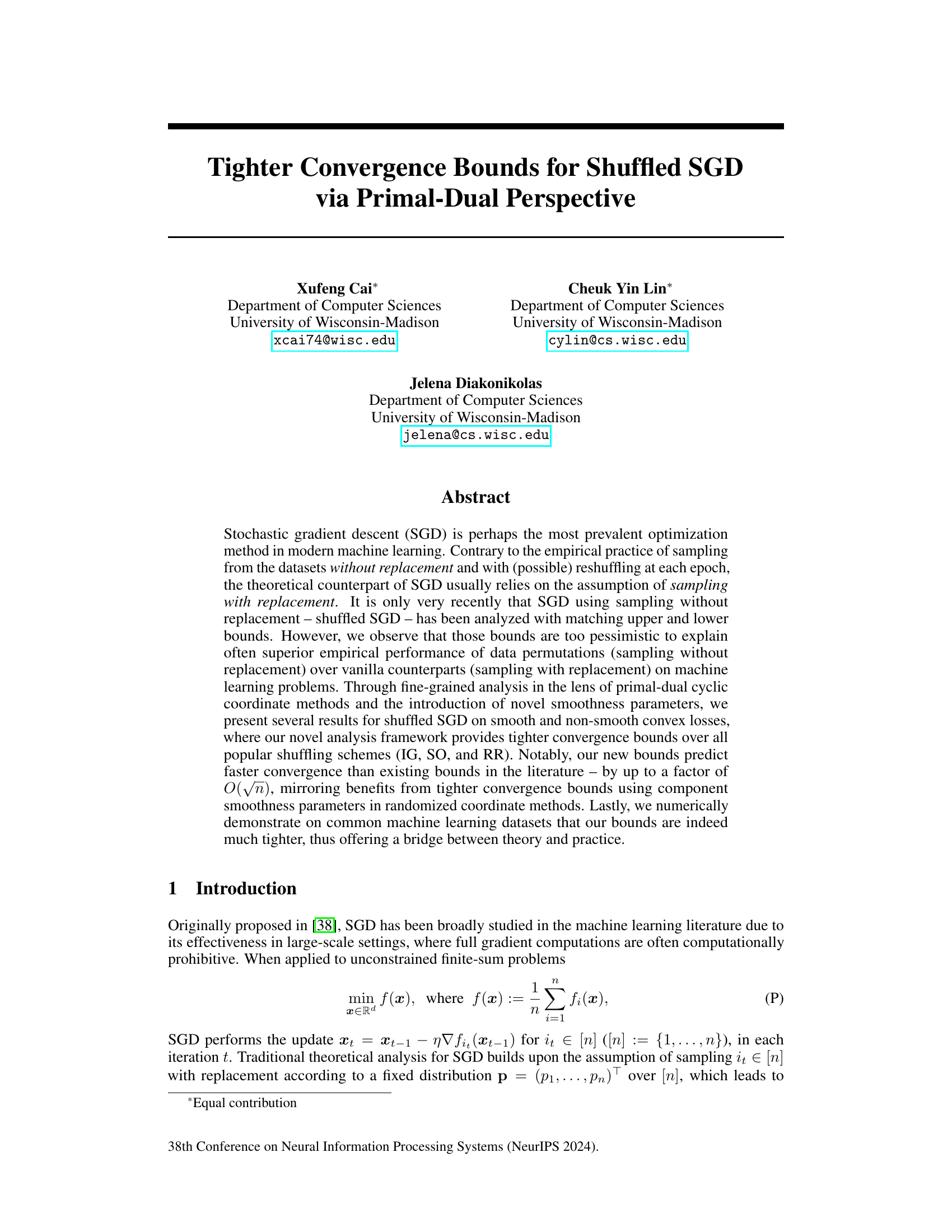
🔼 This figure shows the convergence behavior of shuffled SGD for logistic regression problems using different step sizes. The step sizes used are from both existing theoretical bounds and the bounds proposed in this paper. The results are averaged over 20 runs to account for randomness in the algorithm. The error bars are not visible due to the low variance observed in the results.

read the caption

Figure 1: An illustration of the convergence behaviour of shuffled SGD for logistic regression problems on LIBSVM datasets luke, leu and a9a, where we use step sizes from existing bounds and our work. Due to randomness, we average over 20 runs for each plot and include a ribbon around each line to show its variance. However, as suggested by the concentration of ÎL (see Section 4.1 and Appendix E), the variance across multiple runs is negligible, hence the ribbons are not observable.

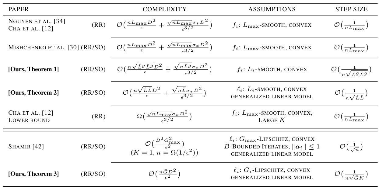
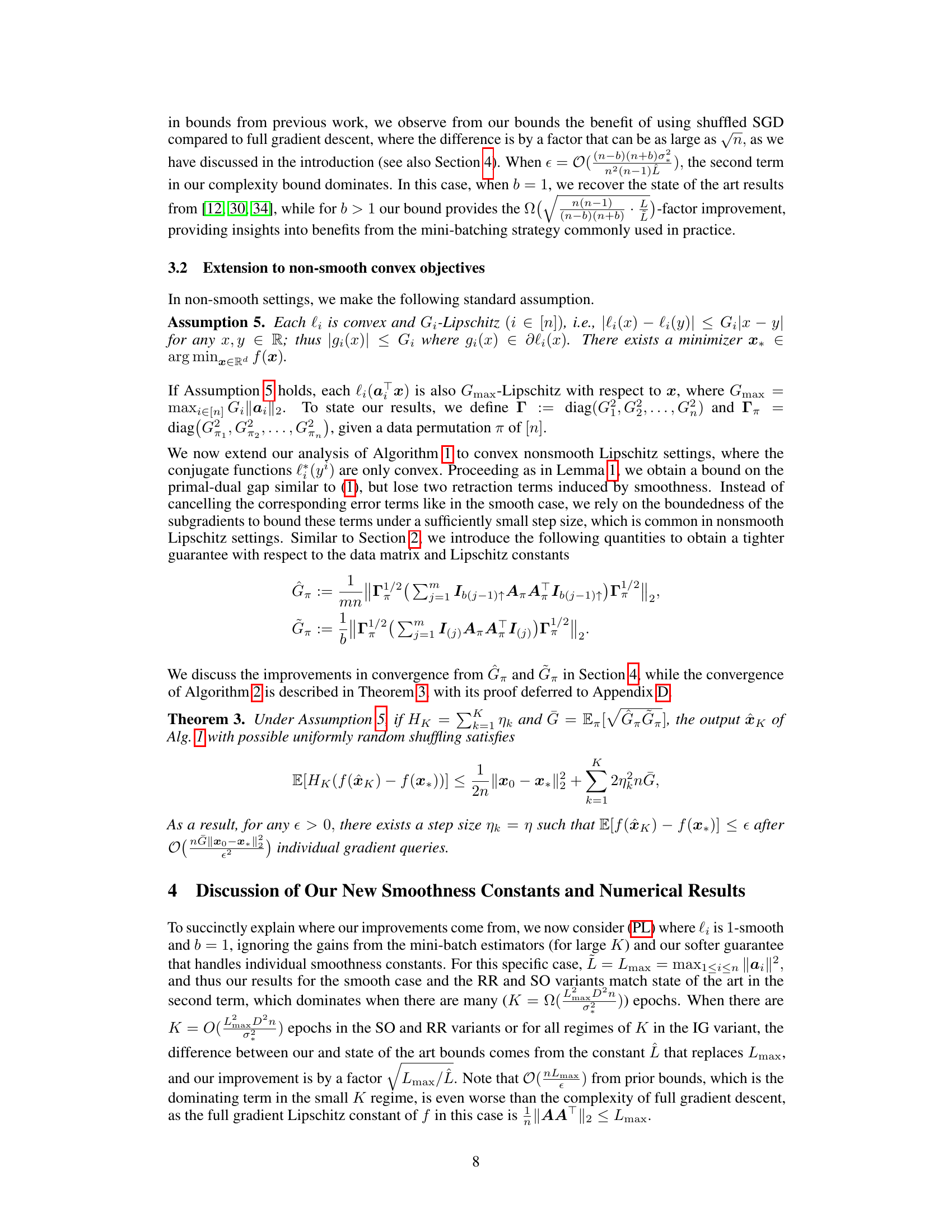
🔼 This table compares the convergence rate results of the proposed method with those of the existing methods in terms of the individual gradient oracle complexity required to achieve a target error. The assumptions made and the step size used for each method are also listed. The table highlights the superior convergence rate obtained by the proposed method, especially in the generalized linear model setting. The table uses parameters defined and discussed within the paper.

read the caption

Table 1: Comparison of our results with state of the art, in terms of individual gradient oracle complexity required to output xout with E[f(xout) - f(x*)] < €, where € > 0 is the target error and x* is the optimal solution. Here, σ² = 1/n Σn=1 ||∇fi(x*)||2, D = ||x0 - x*||2, and generalized linear model refers to objectives of the form f(x) = Σn=1 li(aTx) as defined in Section 3. Parameters Lº, Lº are defined in Section 2 and satisfy Lº < Σn=1 Li and Lº < Lmax. Parameters L, L, and G are defined in Section 3, and are discussed in the text of this section.

In-depth insights

#

Shuffled SGD Bounds

#

Analyzing shuffled SGD bounds reveals crucial insights into the optimization landscape. Tightening these bounds is paramount, bridging the gap between theoretical predictions and empirical observations. The primal-dual perspective offers a powerful framework for this analysis, revealing connections to cyclic coordinate methods and enabling the incorporation of fine-grained smoothness parameters. These parameters capture data-dependent structure, leading to improved bounds that predict faster convergence rates, potentially by a factor of O(√n). The analysis extends beyond smooth convex losses to encompass non-smooth settings, further enhancing the theoretical understanding. Numerical experiments validate the improved bounds, showing a significant reduction in the gap between theoretical predictions and practical performance. The study’s success highlights the significance of considering the data’s structure and properties when developing and analyzing optimization algorithms, moving beyond overly simplistic assumptions to produce more accurate and useful results. Future work could explore extensions to more complex settings and further investigate the interplay between algorithm design, data characteristics, and convergence behavior.

Primal-Dual Analysis

#

Primal-dual analysis offers a powerful lens for examining optimization algorithms, particularly stochastic gradient descent (SGD). By viewing the problem through both primal and dual perspectives, we gain a deeper understanding of the algorithm’s dynamics and convergence behavior. This approach allows us to leverage the properties of both the primal objective function and its dual counterpart, potentially leading to tighter convergence bounds and more efficient algorithms. A key advantage is the ability to analyze the algorithm’s progress through the dual space, providing insights into the algorithm’s behavior that are not readily apparent from a purely primal perspective. This dual perspective is crucial, especially in situations where the primal problem is non-smooth or high-dimensional. Moreover, primal-dual analysis allows us to design algorithms that exploit the structure of the problem, leading to more efficient and robust optimization methods. This technique can reveal important relationships between algorithm parameters and problem characteristics, and might unveil new insights into existing methods, thus improving the theoretical understanding and practical performance of SGD and related algorithms.

Smoothness Measures

#

Smoothness measures are crucial for analyzing the convergence rate of optimization algorithms, especially in the context of stochastic gradient descent (SGD). The choice of smoothness measure significantly impacts the theoretical bounds derived. A fine-grained analysis might consider component-wise smoothness parameters, capturing variations in the smoothness of individual loss functions within a dataset. This approach can lead to tighter convergence bounds than those obtained using a global smoothness parameter. The trade-off lies in the increased complexity of calculating component-wise smoothness, compared to using a single, easily computed global parameter. Data-dependent smoothness measures could further refine the analysis, leveraging the specific structure of the training data to create even more accurate convergence guarantees. However, this involves more intricate analysis and might lead to bounds that are less interpretable. The ideal smoothness measure is one that balances theoretical tightness with practical computability and provides valuable insights into the convergence behavior.

Linear Predictors

#

The concept of “Linear Predictors” within machine learning signifies models where the prediction is a linear function of the input features. This linearity implies a direct, proportional relationship between inputs and outputs, often represented by a weighted sum of features. Simplicity is a key advantage, making these models computationally efficient and easily interpretable. However, this simplicity comes at the cost of limited expressiveness. Linear predictors struggle to capture complex, non-linear relationships within data, leading to potentially inaccurate predictions in scenarios demanding more sophisticated modeling. Model enhancements, such as regularization techniques or feature engineering, can improve performance by mitigating overfitting or incorporating non-linear interactions, respectively. Despite limitations, linear predictors serve as foundational building blocks in many advanced machine learning techniques, providing a starting point for more complex models and enabling rapid prototyping and analysis. Their interpretability is especially valuable when understanding model behavior is crucial. The choice of linear predictors represents a trade-off between model complexity, computational efficiency, and predictive power, which must be carefully evaluated within the specific context of the application.

Future Directions

#

The heading ‘Future Directions’ in a research paper would ideally explore promising avenues for extending the current work. For a paper on shuffled SGD, this section could discuss extending the theoretical analysis to more complex settings, such as non-convex or stochastic optimization problems. It would be beneficial to investigate the impact of different data distributions and problem structures on the performance of shuffled SGD, and explore how these findings might lead to improved algorithm design. Furthermore, a thoughtful discussion of practical considerations, such as efficient mini-batching strategies and adaptive step size selection, could significantly enhance the paper’s value. Finally, exploring connections between shuffled SGD and other optimization methods could uncover new insights and potentially lead to hybrid algorithms with superior convergence properties. Ultimately, a strong ‘Future Directions’ section would not simply list ideas, but rather provide a well-reasoned perspective on the most impactful and promising areas for future research.

More visual insights

#

More on figures

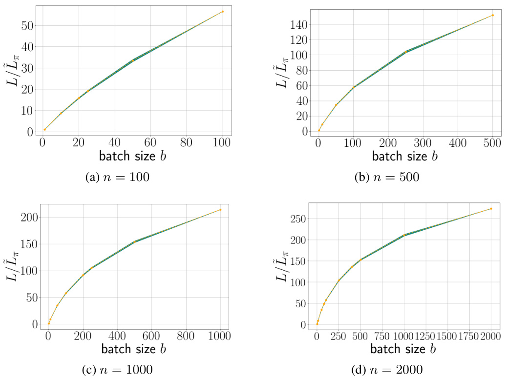
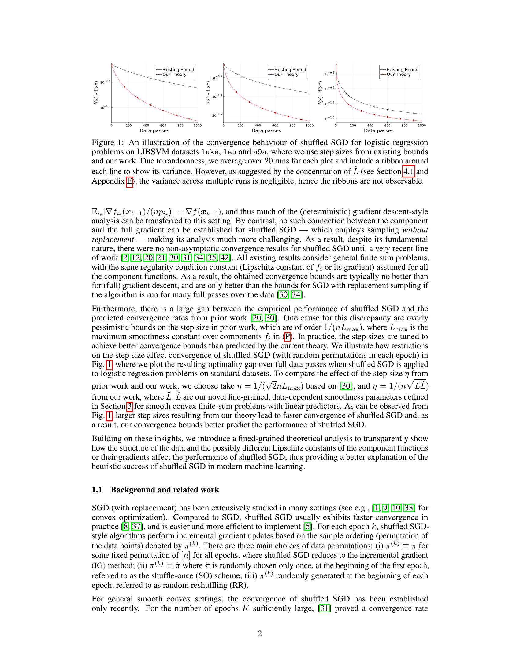
🔼 The figure shows the convergence behavior of shuffled SGD using different step sizes on three LIBSVM datasets. The step sizes used are derived from existing bounds and from the authors’ proposed theoretical work. The plots show the optimality gap versus the number of data passes. Averaging across 20 runs helps smooth out the inherent randomness of the algorithm. The nearly invisible ribbons around the lines demonstrate the negligible variance in the results.

read the caption

Figure 1: An illustration of the convergence behaviour of shuffled SGD for logistic regression problems on LIBSVM datasets luke, leu and a9a, where we use step sizes from existing bounds and our work. Due to randomness, we average over 20 runs for each plot and include a ribbon around each line to show its variance. However, as suggested by the concentration of ÎL (see Section 4.1 and Appendix E), the variance across multiple runs is negligible, hence the ribbons are not observable.

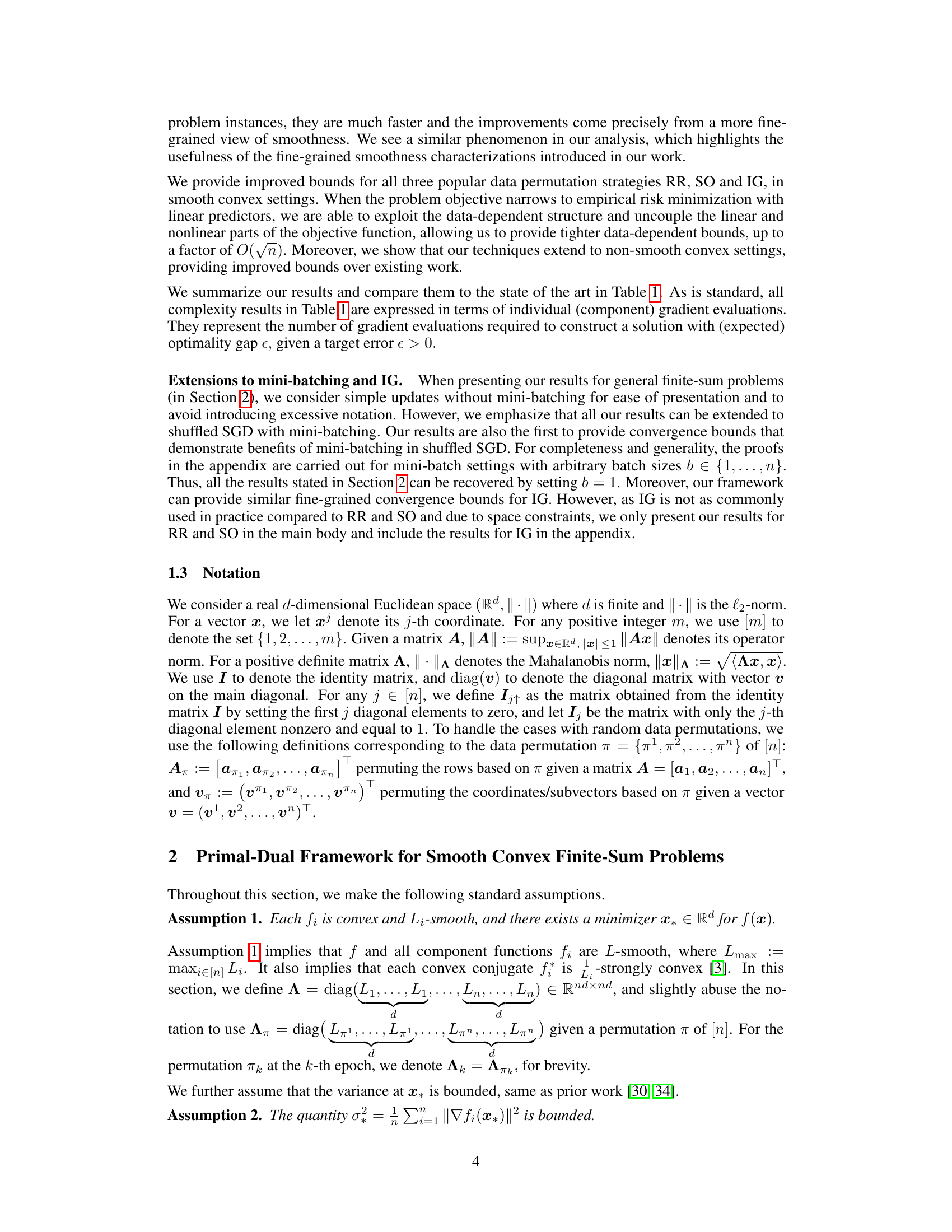
🔼 The figure shows the convergence behavior of shuffled SGD for logistic regression problems on three LIBSVM datasets using step sizes from existing bounds and the proposed method. The results are averaged over 20 runs to account for randomness, with error ribbons indicating variability. The negligible variability supports the claim that the new bounds are tighter and predict faster convergence.

read the caption

Figure 1: An illustration of the convergence behaviour of shuffled SGD for logistic regression problems on LIBSVM datasets luke, leu and a9a, where we use step sizes from existing bounds and our work. Due to randomness, we average over 20 runs for each plot and include a ribbon around each line to show its variance. However, as suggested by the concentration of ÎL (see Section 4.1 and Appendix E), the variance across multiple runs is negligible, hence the ribbons are not observable.

Full paper

#