TL;DR#
Graph Neural Networks (GNNs) often utilize normalization layers originally designed for other data types. These layers fail to capture graph data’s unique characteristics, potentially limiting GNN performance. Existing graph-specific normalization methods also lack consistent benefits.
This paper introduces GRANOLA, a novel graph-adaptive normalization layer. GRANOLA leverages the propagation of random node features (RNF) to generate expressive node representations, allowing it to adapt to each graph’s unique structure. Extensive experiments show that GRANOLA significantly and consistently outperforms existing methods across various benchmarks and architectures. The method’s superior performance is achieved without increasing the computational complexity of message-passing neural networks (MPNNs).
Key Takeaways#
Why does it matter?#
This paper is crucial for researchers in graph neural networks (GNNs) as it directly addresses the limitations of existing normalization techniques and proposes a novel, highly effective solution. GRANOLA’s superior performance across diverse benchmarks and consistent improvement over existing methods highlight its practical significance. This work opens up new avenues for research on GNN normalization, potentially leading to more expressive and efficient GNN architectures.
Visual Insights#

🔼 This figure illustrates different normalization layers used in graph neural networks, showing how they compute statistics across different dimensions of the input data (batch size, number of nodes, number of channels). The colored blue elements highlight the specific components used in the calculations for each normalization method.
read the caption
Figure 1: Illustration of normalization layers. We denote by B, N and C the number of graphs (batch size), nodes, and channels (node features), respectively. For simplicity of presentation, we use the same number of nodes for all graphs. We color in blue the elements used to compute the statistics employed inside the normalization layer.
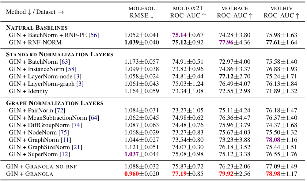
🔼 This table compares GRANOLA’s performance against various baselines on the MOLESOL, MOLTOX21, MOLBACE, and MOLHIV datasets. The baselines include natural baselines (methods using RNFs), standard normalization layers (BatchNorm, InstanceNorm, LayerNorm), and graph-specific normalization layers (PairNorm, MeanSubtractionNorm, etc.). The results demonstrate GRANOLA’s superior performance, consistently achieving top-three rankings across all datasets. The table highlights the impact of RNFs and graph adaptivity, illustrating GRANOLA’s effectiveness compared to methods that lack these features.
read the caption
Table 2: A comparison to natural baselines, standard and graph normalization layers, demonstrating the practical advantages of GRANOLA. The top three methods are marked by First, Second, Third.
In-depth insights#
Adaptive Normalization#
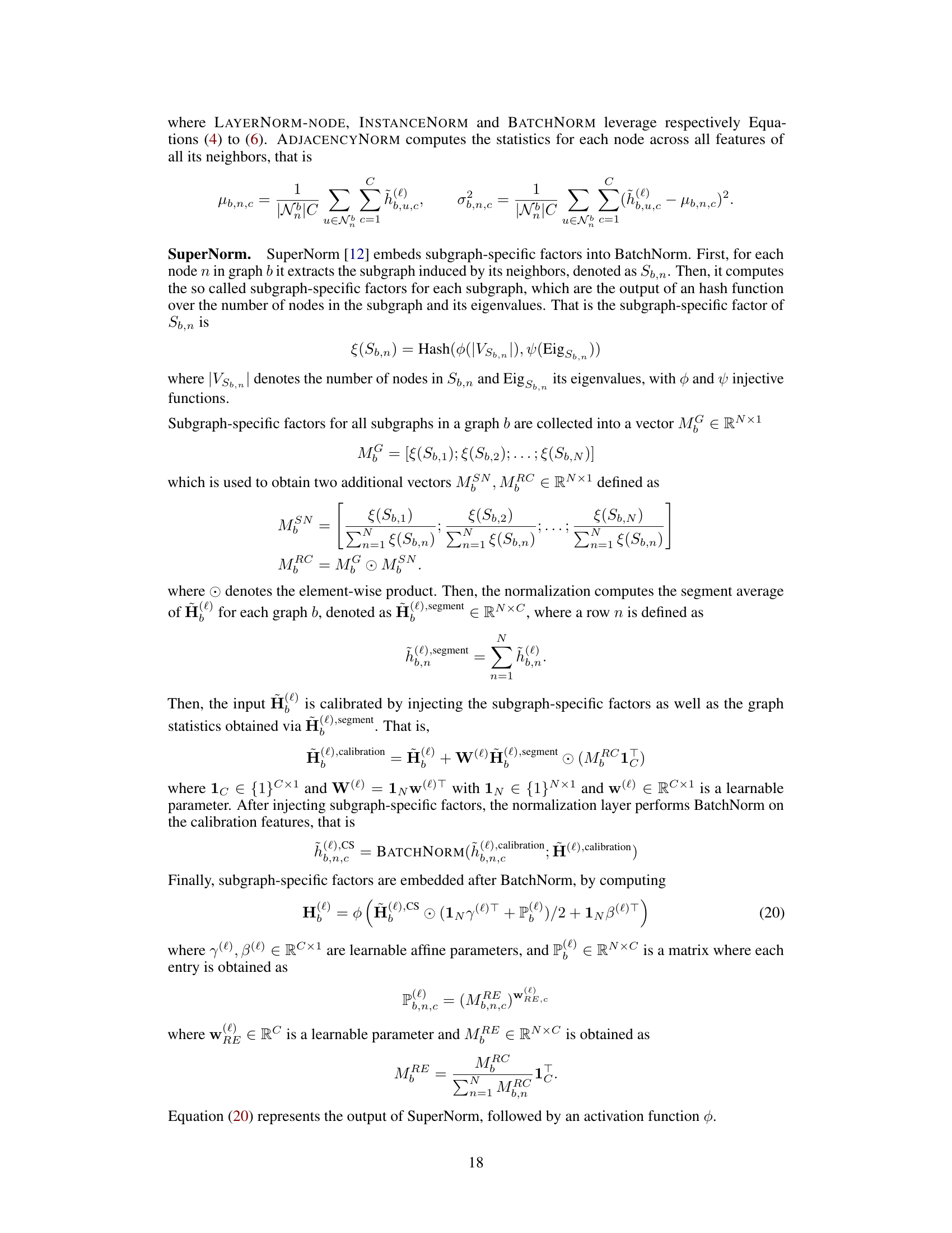
Adaptive normalization techniques aim to enhance the performance of graph neural networks (GNNs) by dynamically adjusting normalization parameters based on the input graph’s structure. Existing normalization methods, often borrowed from other domains, often fail to fully capture the unique characteristics of graph data, potentially hindering GNN performance and expressiveness. Adaptive normalization addresses this by learning graph-specific parameters. This approach leads to more effective normalization, particularly beneficial for tasks where graph structure significantly influences results. A key challenge lies in designing normalization methods capable of learning expressive graph representations while maintaining computational efficiency. Successful adaptive methods often employ additional graph neural network layers to learn these adaptable normalization parameters. While promising results have been observed, further research is needed to address limitations, including the consistent superior performance compared to baselines and the potential trade-off between expressiveness and computational cost.
GRANOLA Framework#
The GRANOLA framework introduces a novel graph-adaptive normalization layer for Graph Neural Networks (GNNs). Addressing the limitations of existing normalization methods, GRANOLA’s key innovation lies in its adaptivity to the input graph’s structure. This adaptivity is achieved through the use of Random Node Features (RNFs) to generate expressive node representations, which are then leveraged to dynamically adjust node features. This method contrasts with previous normalization techniques by avoiding the use of fixed parameters for all nodes. Theoretical analysis demonstrates GRANOLA’s full adaptivity to the graph structure and its improved expressive power, resulting in consistent performance improvements across benchmarks and architectures. The method is especially effective in resolving the oversmoothing issues present in many GNNs, maintaining a time complexity comparable to standard MPNNs. GRANOLA’s superior performance highlights the importance of incorporating graph-specific characteristics in normalization layers. It significantly outperforms existing techniques and establishes itself as a leading normalization approach within the MPNN family.
Expressive Power#
The concept of “Expressive Power” in the context of Graph Neural Networks (GNNs) centers on a model’s capacity to represent complex relationships within graph-structured data. A GNN with high expressive power can capture intricate patterns and features that are difficult for less powerful models to discern. This paper highlights the limitations of existing normalization methods, demonstrating that their off-the-shelf application to GNNs may hinder expressive power. The authors argue that adaptivity to the specific input graph is crucial for effective normalization layers, emphasizing that this necessitates architectures that can fully capture the graph’s unique characteristics. GRANOLA, the proposed method, is designed to maximize expressive power through its utilization of Random Node Features and a powerful normalization GNN. This ensures the model’s adaptivity to different graph structures. The paper’s theoretical analysis provides a rigorous justification for these design choices, demonstrating that GRANOLA is indeed fully adaptive and inherits the expressive power of the underlying architecture. Empirical results validate the superiority of GRANOLA over existing normalization techniques, underscoring its ability to enhance the expressive power of GNNs and lead to significant performance improvements across various tasks and datasets.
Empirical Evaluation#
An Empirical Evaluation section in a research paper would rigorously assess the proposed method’s performance. This would involve comparing it against relevant baselines on a variety of datasets, using standard metrics to quantify performance. A strong evaluation would include a detailed analysis of these results, considering factors like dataset characteristics, computational cost, and statistical significance. It’s crucial to address potential limitations and biases, demonstrating the method’s robustness and generalizability. Visualizations, such as graphs or tables, are essential to effectively communicate the results. Statistical testing would provide confidence in the findings, while ablation studies could isolate the contribution of individual components. The ultimate goal is to present compelling evidence showcasing the method’s advantages and identifying areas for future work, establishing its value within the existing research landscape. A comprehensive evaluation is essential for building trust and ensuring the reliability of any scientific contribution.
Future Directions#
Future research could explore several promising avenues. Extending GRANOLA to other GNN architectures beyond those tested would broaden its applicability and demonstrate its robustness. Investigating alternative normalization GNNs within GRANOLA, beyond the MPNNs used here, could potentially enhance performance or efficiency. A thorough analysis of GRANOLA’s behavior in the presence of noisy or incomplete graph data is crucial to understand its limitations and improve its resilience. Developing a more efficient implementation of GRANOLA, potentially through architectural modifications or algorithmic improvements, is needed to address scalability concerns for very large graphs. Finally, exploring theoretical connections between GRANOLA and other expressive GNN architectures could provide valuable insights into the fundamental limitations and capabilities of current GNN technology.
More visual insights#
More on figures
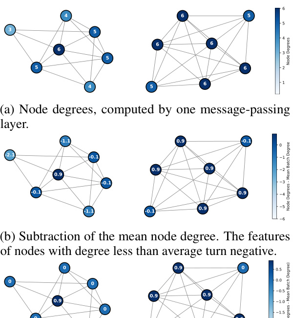
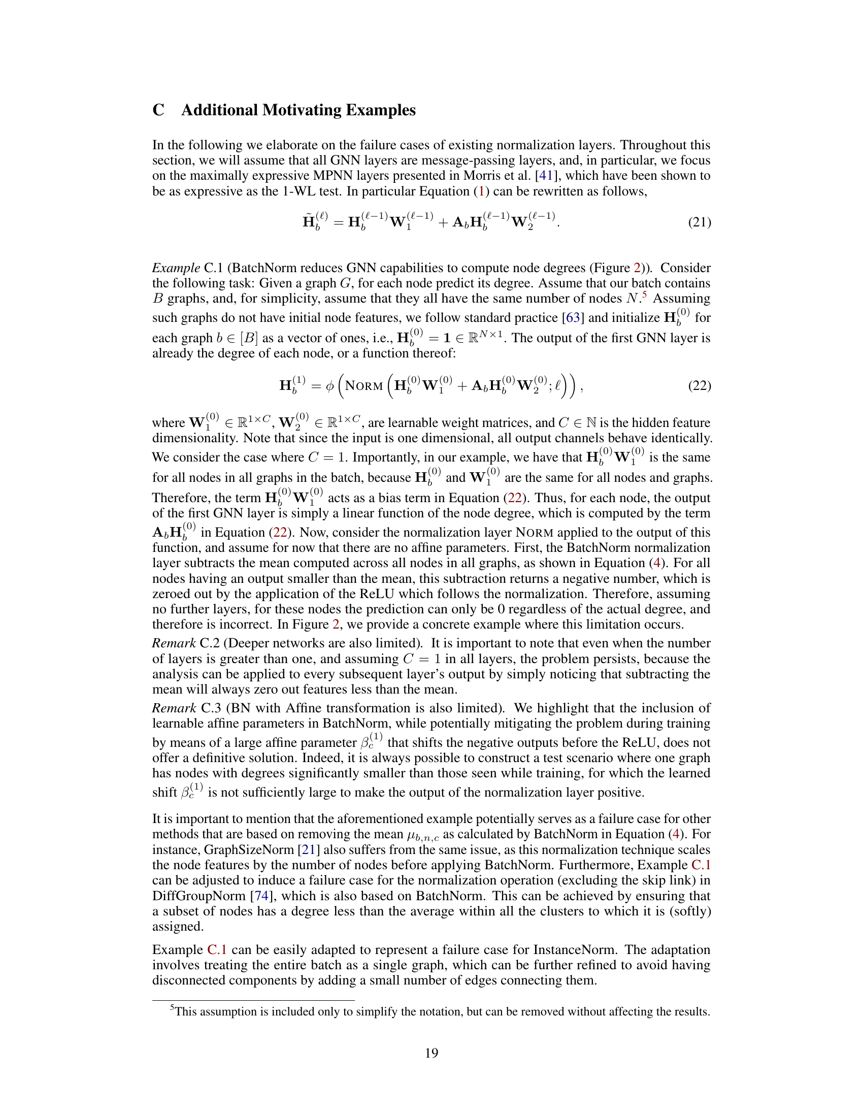
🔼 This figure shows an example illustrating the limitations of BatchNorm and similar normalization methods. It demonstrates that when subtracting the mean computed across the batch, the features of nodes with degrees less than the average turn negative, which are then set to 0 by the ReLU activation function, thus hindering the prediction of the node degrees.
read the caption
Figure 2: A batch of two graphs, where subtracting the mean of the node features computed across the batch, as in BatchNorm and related methods, results in the loss of capacity to compute node degrees.

🔼 This figure illustrates the architecture of the GRANOLA layer. It takes as input the node features from the previous layer (H(l−1)) and the adjacency matrix (Ab) of the graph. These inputs are processed by a GNN layer (GNNLAYER) to produce intermediate node features (Ĥ(l)). Simultaneously, random node features (R(l)b) are sampled and, along with Ĥ(l) and Ab, fed into a normalization GNN (GNNNORM). The normalization GNN outputs the normalization parameters (γ(l)b,n, β(l)b,n), which are then used to normalize the intermediate features (Ĥ(l)) resulting in the final normalized features (H(l)). The inclusion of random node features is crucial for achieving full adaptivity of the normalization to the input graph structure.
read the caption
Figure 3: Illustration of a GRANOLA layer. Given node features Ĥ(l−1) and the adjacency matrix Ab, we feed them to a GNNLAYER to extract intermediate node features Ĥ(l). Then, we predict normalization parameters using GNNNORM, which takes sampled RNF R(l)b, Ĥ(l), Ab. Including R(l)b with Ab and Ĥ(l) enhances the expressiveness of GRANOLA ensuring full adaptivity.

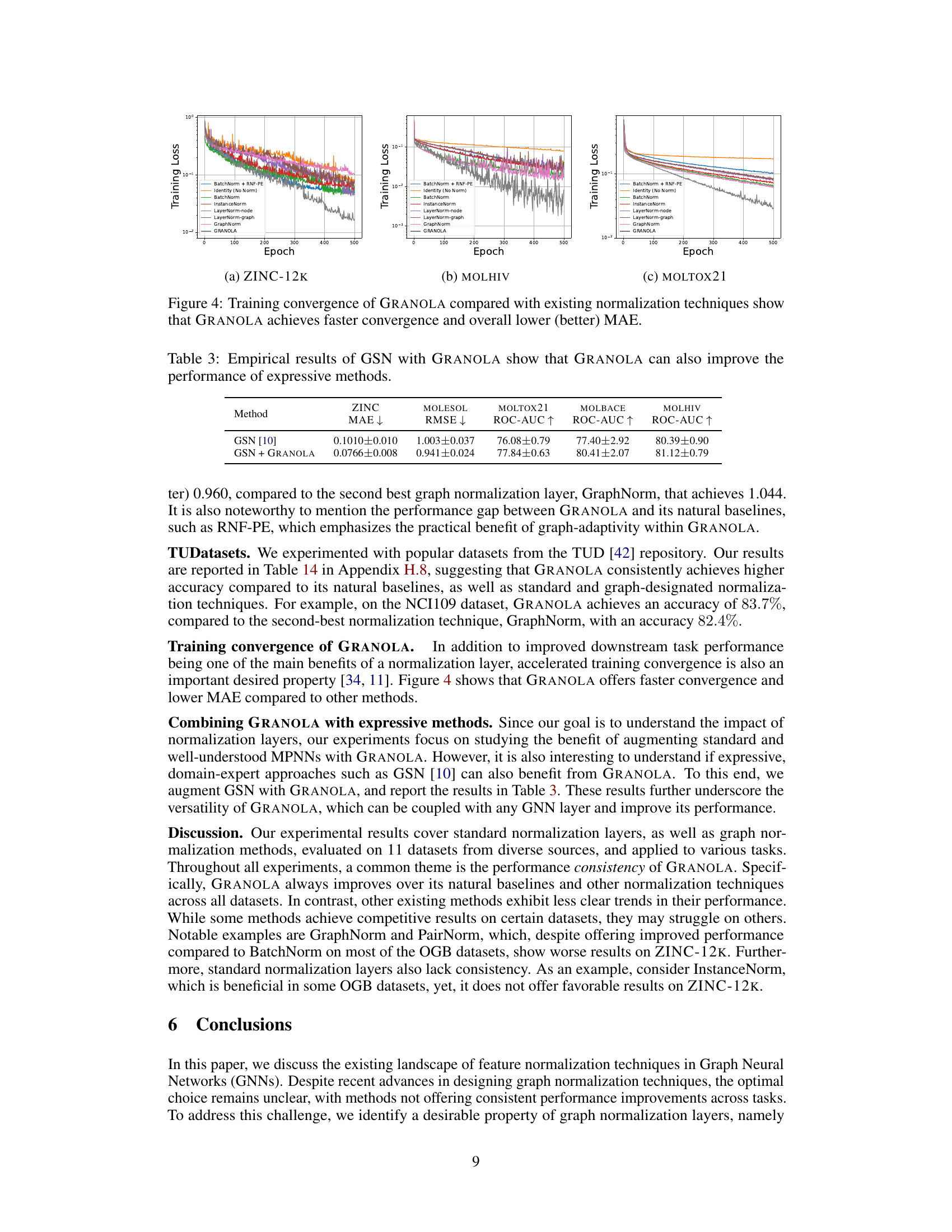
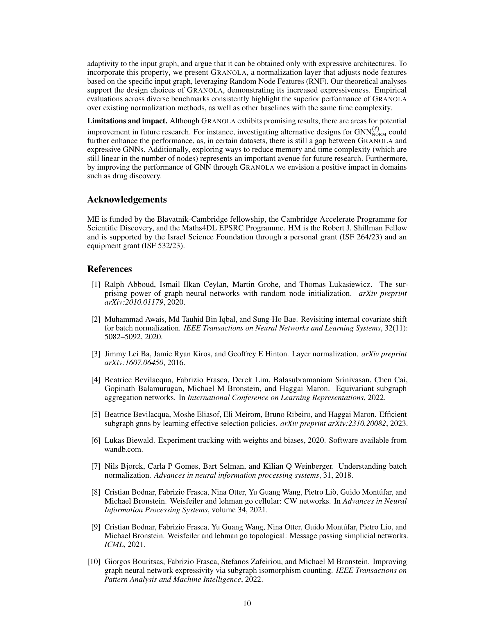
🔼 This figure shows the training loss curves for various normalization methods, including GRANOLA, across three different datasets: ZINC-12K, MOLHIV, and MOLTOX21. The plots demonstrate that GRANOLA consistently achieves faster convergence (reaching a lower loss in fewer epochs) and ultimately lower training loss (mean absolute error, or MAE) than competing normalization techniques.
read the caption
Figure 4: Training convergence of GRANOLA compared with existing normalization techniques show that GRANOLA achieves faster convergence and overall lower (better) MAE.

🔼 This figure shows an example demonstrating the limitations of BatchNorm and similar methods (that subtract the mean across all nodes) in graph neural networks. Two graphs are displayed: one with nodes having degrees 1 and 2, and another with nodes having degrees 1 and 3. When the mean node degree is subtracted, nodes with degrees less than the mean have negative values. Because of the ReLU activation function commonly used in GNNs, the negative values become 0, losing the information about the original node degree and preventing the network from accurately learning node degree prediction. This highlights the need for adaptive normalization techniques in GNNs.
read the caption
Figure 2: A batch of two graphs, where subtracting the mean of the node features computed across the batch, as in BatchNorm and related methods, results in the loss of capacity to compute node degrees.

🔼 This figure shows two graphs where BatchNorm (or similar methods) is applied. (a) shows node degrees after a message-passing layer. (b) shows the result after subtracting the mean node degree across both graphs. Features of nodes with lower than average degrees become negative. (c) shows that after applying a ReLU activation, all negative values are set to zero, hindering the ability of the network to distinguish between nodes with different degrees.
read the caption
Figure 2: A batch of two graphs, where subtracting the mean of the node features computed across the batch, as in BatchNorm and related methods, results in the loss of capacity to compute node degrees.
More on tables
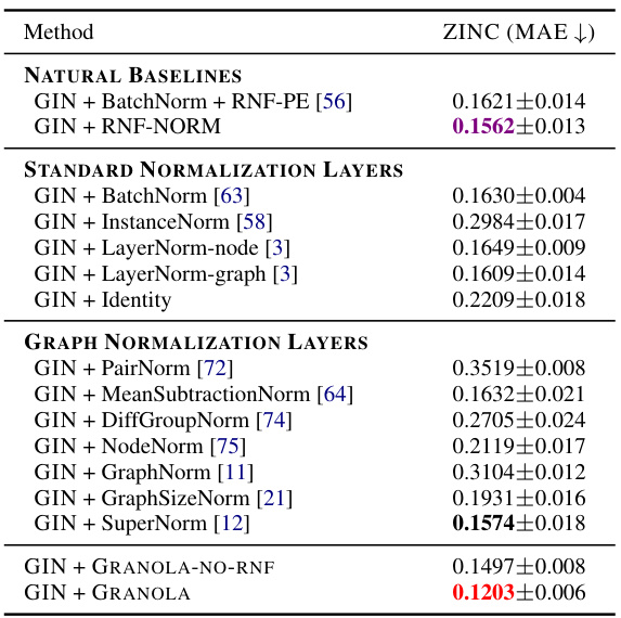
🔼 This table presents a comparison of GRANOLA’s performance against various baseline methods on the ZINC-12K dataset. The baselines include standard normalization layers (BatchNorm, InstanceNorm, LayerNorm variants, Identity), graph-specific normalization layers (PairNorm, MeanSubtractionNorm, DiffGroupNorm, NodeNorm, GraphNorm, GraphSizeNorm, SuperNorm), and GRANOLA’s variants (GRANOLA-NO-RNF). All methods are constrained to a 500k parameter budget. The table highlights GRANOLA’s superior performance by marking the top three performing methods.
read the caption
Table 1: Comparison of GRANOLA with various baselines on the ZINC-12K dataset. All methods obey to the 500k parameter budget. The top three methods are marked by First, Second, Third.

🔼 This table presents a comprehensive comparison of GRANOLA against various baselines on multiple molecular datasets. It compares GRANOLA’s performance against natural baselines (methods that incorporate random node features), standard normalization layers (BatchNorm, InstanceNorm, LayerNorm), graph-specific normalization methods (PairNorm, MeanSubtractionNorm, DiffGroupNorm, NodeNorm, GraphNorm, GraphSizeNorm, SuperNorm), and two variants of GRANOLA itself (GRANOLA-NO-RNF, which omits random node features, and GRANOLA-MS, a simplified version). The results show GRANOLA’s superior performance across different metrics (RMSE, ROC-AUC) and datasets, highlighting its practical advantages over existing methods.
read the caption
Table 2: A comparison to natural baselines, standard and graph normalization layers, demonstrating the practical advantages of GRANOLA. The top three methods are marked by First, Second, Third.

🔼 This table compares GRANOLA’s performance against various baselines across four molecular datasets (MOLESOL, MOLTOX21, MOLBACE, MOLHIV). The baselines include natural baselines (methods using RNF but not GRANOLA’s graph-adaptive approach), standard normalization layers (BatchNorm, InstanceNorm, LayerNorm variants), and graph-specific normalization layers (PairNorm, MeanSubtractionNorm, DiffGroupNorm, NodeNorm, GraphNorm, GraphSizeNorm, SuperNorm). The results show GRANOLA’s superior performance across different datasets and normalization methods. The top three performing methods for each dataset are highlighted.
read the caption
Table 2: A comparison to natural baselines, standard and graph normalization layers, demonstrating the practical advantages of GRANOLA. The top three methods are marked by First, Second, Third.

🔼 This table presents a comparison of GRANOLA’s performance against various baselines on the MOL* datasets from the Open Graph Benchmark (OGB). The baselines include natural baselines (methods using random node features (RNF)), standard normalization layers (BatchNorm, InstanceNorm, LayerNorm variants), and graph-specific normalization layers. The table shows the RMSE and ROC-AUC scores for each method across the MOL* datasets. The top three performing methods for each dataset are highlighted.
read the caption
Table 2: A comparison to natural baselines, standard and graph normalization layers, demonstrating the practical advantages of GRANOLA. The top three methods are marked by First, Second, Third.

🔼 This table compares GRANOLA’s performance against various baselines on the ZINC-12K and OGB datasets for molecular property prediction tasks. It shows GRANOLA’s RMSE and ROC-AUC scores alongside baselines that include standard normalization layers (BatchNorm, InstanceNorm, LayerNorm), graph-specific normalization layers (PairNorm, MeanSubtractionNorm, etc.), and natural baselines incorporating RNFs. The table highlights GRANOLA’s consistent superior performance and ranks the top three methods across each dataset.
read the caption
Table 2: A comparison to natural baselines, standard and graph normalization layers, demonstrating the practical advantages of GRANOLA. The top three methods are marked by First, Second, Third.

🔼 This table compares the performance of GRANOLA against various baselines across multiple datasets (MOLESOL, MOLTOX21, MOLBACE, MOLHIV). The baselines include natural baselines (methods using RNFs but not full graph adaptivity), standard normalization layers (BatchNorm, InstanceNorm, LayerNorm variants), and graph-specific normalization layers (PairNorm, MeanSubtractionNorm, DiffGroupNorm, NodeNorm, GraphNorm, GraphSizeNorm, SuperNorm). The table shows RMSE and ROC-AUC scores for each method and dataset. The top three performing methods for each dataset are highlighted.
read the caption
Table 2: A comparison to natural baselines, standard and graph normalization layers, demonstrating the practical advantages of GRANOLA. The top three methods are marked by First, Second, Third.

🔼 This table compares GRANOLA’s performance against various baselines on the ZINC-12k and OGB datasets. The baselines include natural baselines (methods that use RNF but lack graph adaptivity), standard normalization layers (BatchNorm, InstanceNorm, LayerNorm), and graph-specific normalization layers. The table reports metrics such as RMSE and ROC-AUC to demonstrate GRANOLA’s superior performance across these different tasks and datasets. The top three performing methods for each dataset are highlighted.
read the caption
Table 2: A comparison to natural baselines, standard and graph normalization layers, demonstrating the practical advantages of GRANOLA. The top three methods are marked by First, Second, Third.

🔼 This table compares GRANOLA’s performance against various baselines across four datasets (MOLESOL, MOLTOX21, MOLBACE, MOLHIV). The baselines include natural baselines (methods using RNFs but without graph adaptivity), standard normalization layers (BatchNorm, InstanceNorm, LayerNorm variants, and Identity), and existing graph-specific normalization layers. The table shows that GRANOLA consistently outperforms all baselines, achieving top-three performance across all datasets, demonstrating its effectiveness and efficiency.
read the caption
Table 2: A comparison to natural baselines, standard and graph normalization layers, demonstrating the practical advantages of GRANOLA. The top three methods are marked by First, Second, Third.
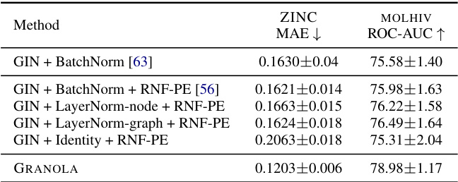
🔼 This table compares GRANOLA’s performance against various baselines on multiple molecular datasets. The baselines include standard normalization techniques (BatchNorm, InstanceNorm, LayerNorm), graph-specific normalization methods (PairNorm, MeanSubtractionNorm, etc.), and methods that incorporate random node features (RNF). The table shows that GRANOLA consistently outperforms other methods across various metrics, often achieving top performance among all baselines, highlighting its effectiveness in graph-structured data.
read the caption
Table 2: A comparison to natural baselines, standard and graph normalization layers, demonstrating the practical advantages of GRANOLA. The top three methods are marked by First, Second, Third.

🔼 This table compares GRANOLA’s performance against various baselines across four molecular datasets. These baselines include methods without normalization, standard normalization techniques (BatchNorm, InstanceNorm, LayerNorm variants), and other graph-specific normalization methods. The results demonstrate GRANOLA’s superior performance across various metrics and datasets, highlighting its practical advantages in graph neural network training.
read the caption
Table 2: A comparison to natural baselines, standard and graph normalization layers, demonstrating the practical advantages of GRANOLA. The top three methods are marked by First, Second, Third.
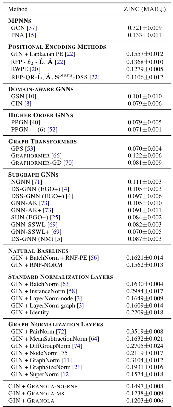
🔼 This table compares GRANOLA’s performance against various baselines on the ZINC-12K and OGB datasets. Baselines include standard normalization techniques (BatchNorm, InstanceNorm, LayerNorm), graph-specific normalization methods, and natural baselines incorporating RNF in different ways. The table shows RMSE and ROC-AUC scores across various datasets, highlighting GRANOLA’s superior performance and ranking it among the top three methods in most cases. The table helps demonstrate the effectiveness of GRANOLA compared to other normalization methods.
read the caption
Table 2: A comparison to natural baselines, standard and graph normalization layers, demonstrating the practical advantages of GRANOLA. The top three methods are marked by First, Second, Third.
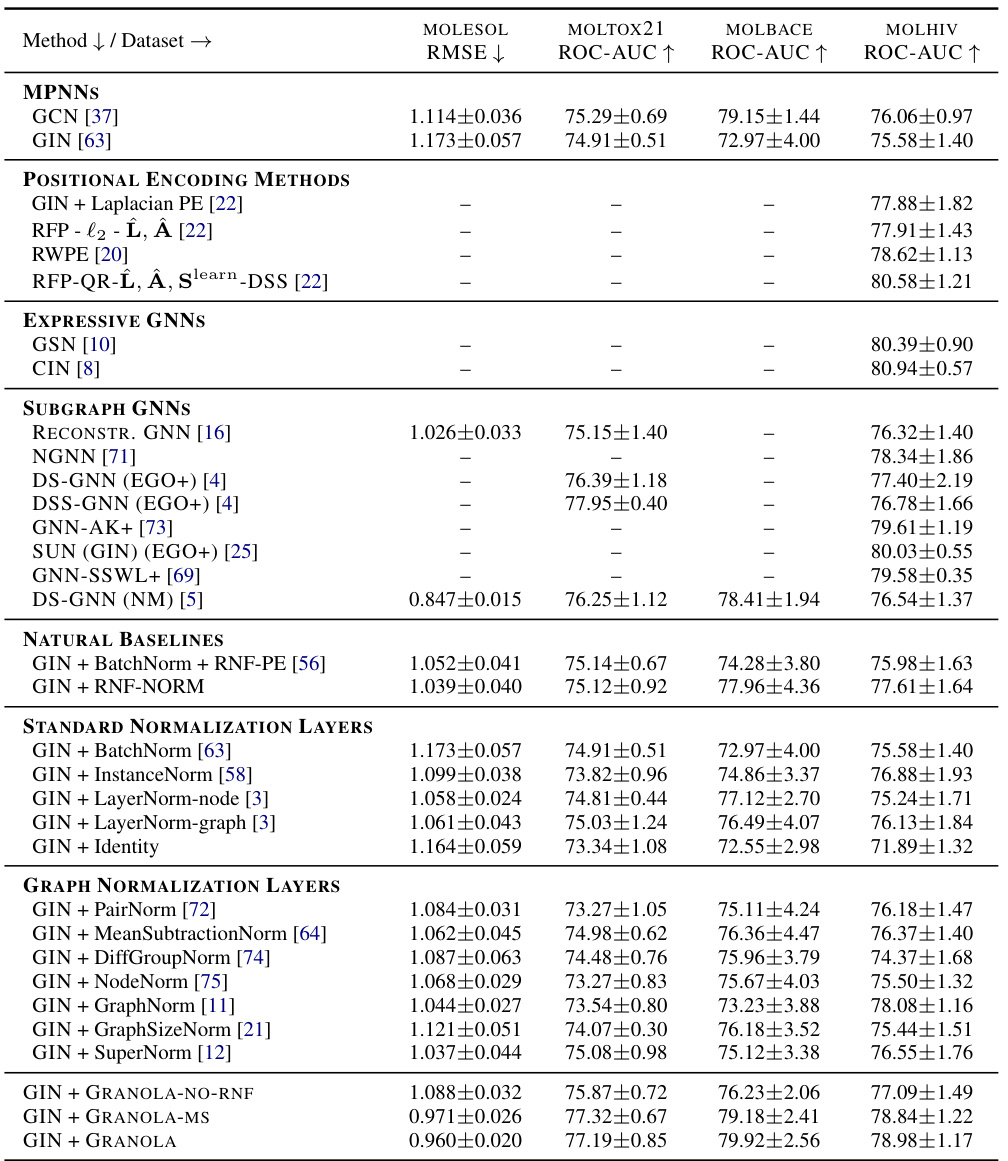
🔼 This table compares GRANOLA’s performance against various baselines on the MOL* datasets from the Open Graph Benchmark (OGB) collection. The baselines include standard normalization techniques (BatchNorm, InstanceNorm, LayerNorm), graph-specific normalization methods (PairNorm, MeanSubtractionNorm, etc.), and natural baselines that incorporate random node features (RNF). The table shows that GRANOLA consistently outperforms other methods, achieving the best results in most cases. The top three performing methods for each dataset are highlighted.
read the caption
Table 2: A comparison to natural baselines, standard and graph normalization layers, demonstrating the practical advantages of GRANOLA. The top three methods are marked by First, Second, Third.

🔼 This table compares GRANOLA’s performance against various baselines across four molecular datasets. The baselines include methods without normalization, standard normalization techniques (BatchNorm, InstanceNorm, LayerNorm), and other graph-specific normalization methods. The table shows that GRANOLA consistently outperforms existing methods across multiple metrics (RMSE and ROC-AUC). The top three performing methods for each dataset and metric are highlighted.
read the caption
Table 2: A comparison to natural baselines, standard and graph normalization layers, demonstrating the practical advantages of GRANOLA. The top three methods are marked by First, Second, Third.
Full paper#

