TL;DR#
Existing time series synthesis methods are limited to generating new series from scratch, either unconditionally or conditionally, and cannot modify existing data while preserving its inherent structure. This paper introduces the novel task of Time Series Editing (TSE), aiming to directly manipulate specific attributes of an input time series while maintaining the original characteristics. The lack of comprehensive data coverage and the complexities of multi-scale attribute-time series relationships are key challenges.
To overcome these challenges, the authors introduce TEdit, a novel diffusion model trained with a bootstrap learning algorithm and a multi-resolution modeling and generation paradigm. The bootstrap learning algorithm enhances the limited data coverage by using generated data for pseudo-supervision. The multi-resolution paradigm effectively captures the intricate relationships between time series and attributes at various scales. Experimental results demonstrate that TEdit successfully edits specified attributes while preserving consistency, outperforming existing methods. A new benchmark dataset is also released.
Key Takeaways#
Why does it matter?#
This paper is important because it introduces a novel task of Time Series Editing (TSE), addressing the limitations of existing time series synthesis methods. It proposes a novel diffusion model, TEdit, that effectively modifies existing time series while preserving other properties. This opens avenues for various applications, particularly in areas with privacy concerns and data scarcity, making it relevant to researchers in time series analysis, machine learning, and related fields. The provided benchmark dataset further facilitates future research in this domain.
Visual Insights#
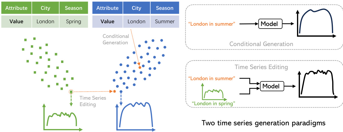
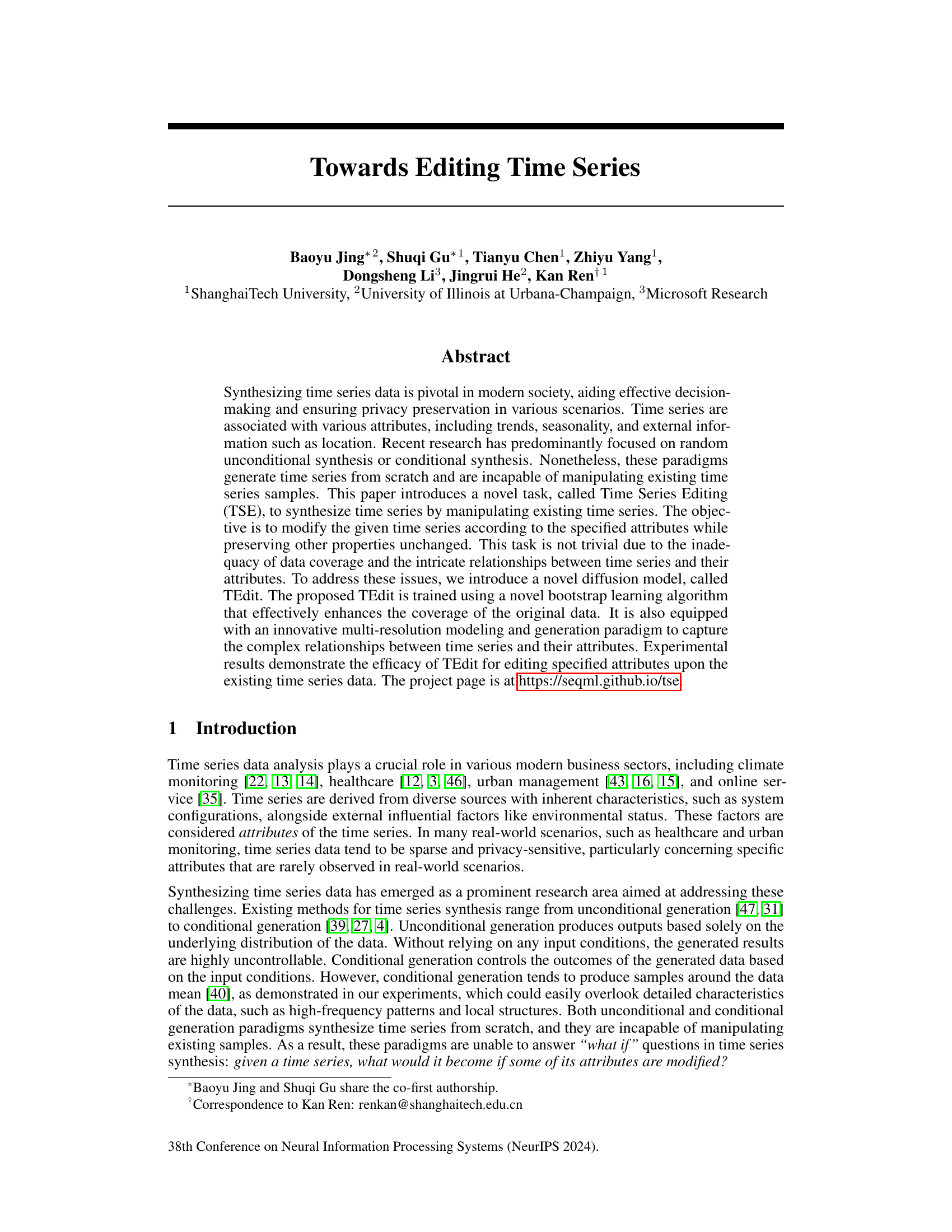
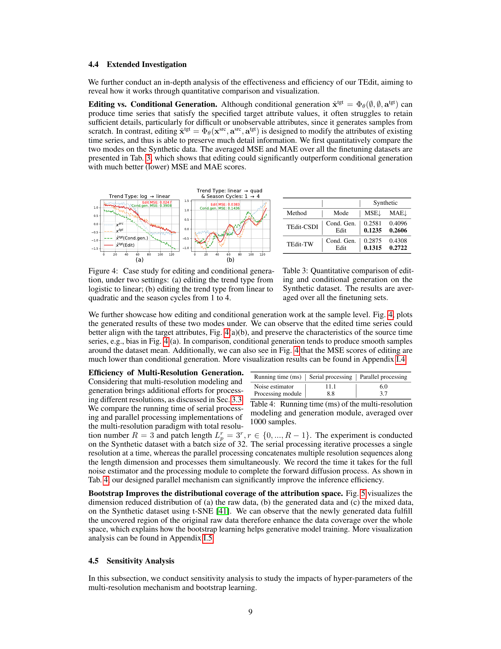
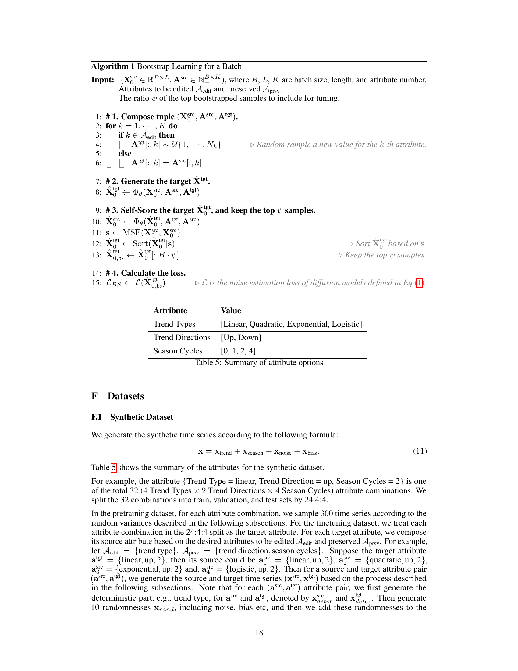
🔼 This figure illustrates the difference between two time series generation paradigms: conditional generation and time series editing. Conditional generation synthesizes time series from scratch, resulting in samples clustered around the data mean. In contrast, time series editing modifies an existing time series sample, adjusting specific attributes to target values while preserving other characteristics. The figure uses the example of air quality in London during spring and summer to visually represent how each method operates.
read the caption
Figure 1: Illustration of the time series generation paradigms. Conditional generation generates time series from scratch, which usually generates samples around the dataset mean. Time series editing allows for the manipulation of the attributes of an input time series sample, which aligns with the desired target attribute values while preserving other properties.

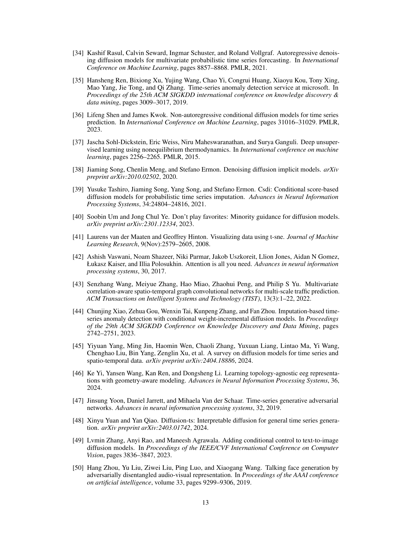
🔼 This table presents the average performance metrics across all finetuning sets for three datasets: Synthetic, Air, and Motor. For each dataset, it shows the overall performance (MSE and MAE), and the performance on both edited and preserved attributes (RaTS, CTAP, |RaTS|, CTAP). The metrics measure the model’s ability to edit specified attributes and maintain consistency in other characteristics. Higher RaTS and CTAP scores indicate better editing, while lower |RaTS| and higher CTAP scores indicate better preservation.
read the caption
Table 1: Averaged performance over all finetuning sets for Synthetic (left), Air (middle), and Motor (right). 'Edited' and 'Preserved' are the average results of all edited and preserved attributes.
In-depth insights#
TSE: A Novel Task#
The heading “TSE: A Novel Task” introduces a significant contribution to the field of time series data manipulation. The authors propose Time Series Editing (TSE), a novel task focusing on modifying existing time series data according to specified attribute changes while preserving other properties. This is a departure from traditional methods that focus on generating time series from scratch. The novelty lies in its direct manipulation of existing data, enabling a unique “what-if” analysis of time series, a capability currently absent in existing techniques. This approach has significant potential in various applications where directly manipulating existing data is advantageous, such as privacy-preserving data synthesis, data augmentation, and counterfactual analysis in areas like climate modelling or healthcare. The success of the TSE task hinges on effectively addressing the challenges inherent in understanding and modeling the intricate relationships between time series data and their diverse attributes, as well as dealing with potential biases in the data distribution. The introduction of TSE as a distinct task opens new avenues of research and application in time series data handling and analysis.
TEdit Diffusion#
TEdit Diffusion, a hypothetical diffusion model for time series editing, presents a novel approach to manipulating existing time series data. Its core innovation lies in directly modifying specified attributes of a given time series while preserving its other inherent characteristics. This contrasts sharply with traditional unconditional and conditional generation methods which synthesize series from scratch. A key challenge addressed is the often sparse and uneven distribution of time series data across attribute spaces, a problem mitigated by a proposed bootstrap learning algorithm that leverages generated data to enhance model training. Furthermore, the model incorporates a multi-resolution paradigm to handle attributes affecting the series at varying scales. While promising, the success of TEdit Diffusion hinges on the effectiveness of both the bootstrap algorithm and the multi-resolution structure in capturing and effectively modeling the complex relationships between time series and their attributes. The model’s performance across various real-world datasets is key to assessing its practical utility and demonstrating its advantages over generating entirely new time series.
Multi-res Editing#
The concept of “Multi-res Editing” in the context of time series manipulation suggests a powerful approach to handling the inherent complexities of temporal data. Different aspects of a time series, such as trends and seasonality, operate at varying resolutions. A multi-resolution approach allows for targeted modifications to specific attributes without disrupting others. For example, a low-resolution edit might adjust an overall trend, while a high-resolution edit could alter a localized anomaly or seasonal pattern. This granular control offers a significant advantage over traditional editing methods that treat the time series uniformly. The effectiveness of this technique hinges on the ability of the model to accurately capture and preserve inter-resolution dependencies. A robust multi-resolution model is crucial for handling such intricate interactions, ensuring that edits at one resolution do not inadvertently introduce unintended artifacts at others. Successfully implementing multi-res editing would have significant implications for numerous applications including forecasting, anomaly detection, and data synthesis, offering the ability to generate more realistic and controlled synthetic time series datasets.
Bootstrap Learning#
Bootstrap learning, in the context of time series editing, is a powerful technique to improve model training by leveraging generated data as pseudo-supervision. It tackles the challenge of limited real-world data coverage, which can hinder the accurate learning of intricate relationships between time series and their attributes. The process involves using the trained diffusion model to create synthetic time series samples, which are then used to augment the training dataset. A key step is a self-scoring mechanism that evaluates the quality of these generated samples by measuring their consistency across various attribute edits. High-confidence samples are selected and added to the training data, effectively boosting data coverage in regions underrepresented in the original dataset. This iterative refinement procedure enhances model generalization and enables the model to learn better from the available data, ultimately improving the editing performance.
Future of TSE#
The future of Time Series Editing (TSE) is bright, promising advancements across various domains. Improved model architectures such as hybrid models combining diffusion and other generative techniques could significantly enhance editing precision and control. Addressing multi-modality within TSE presents exciting opportunities; integrating diverse data types (images, text, sensor data) alongside time series will enrich editing capabilities and enable the creation of more realistic and nuanced synthetic datasets. The need for robust handling of missing or noisy data will likely drive research into more sophisticated imputation techniques, as well as the development of models that are inherently robust to these imperfections. Furthermore, research into more efficient training methods and algorithms is essential to scaling TSE to larger, more complex datasets. Finally, ethical considerations will increasingly shape the future of TSE, necessitating methods that ensure data privacy, fairness, and prevent the misuse of the technology for malicious purposes. Addressing these challenges will unlock TSE’s full potential, transforming numerous applications.
More visual insights#
More on figures

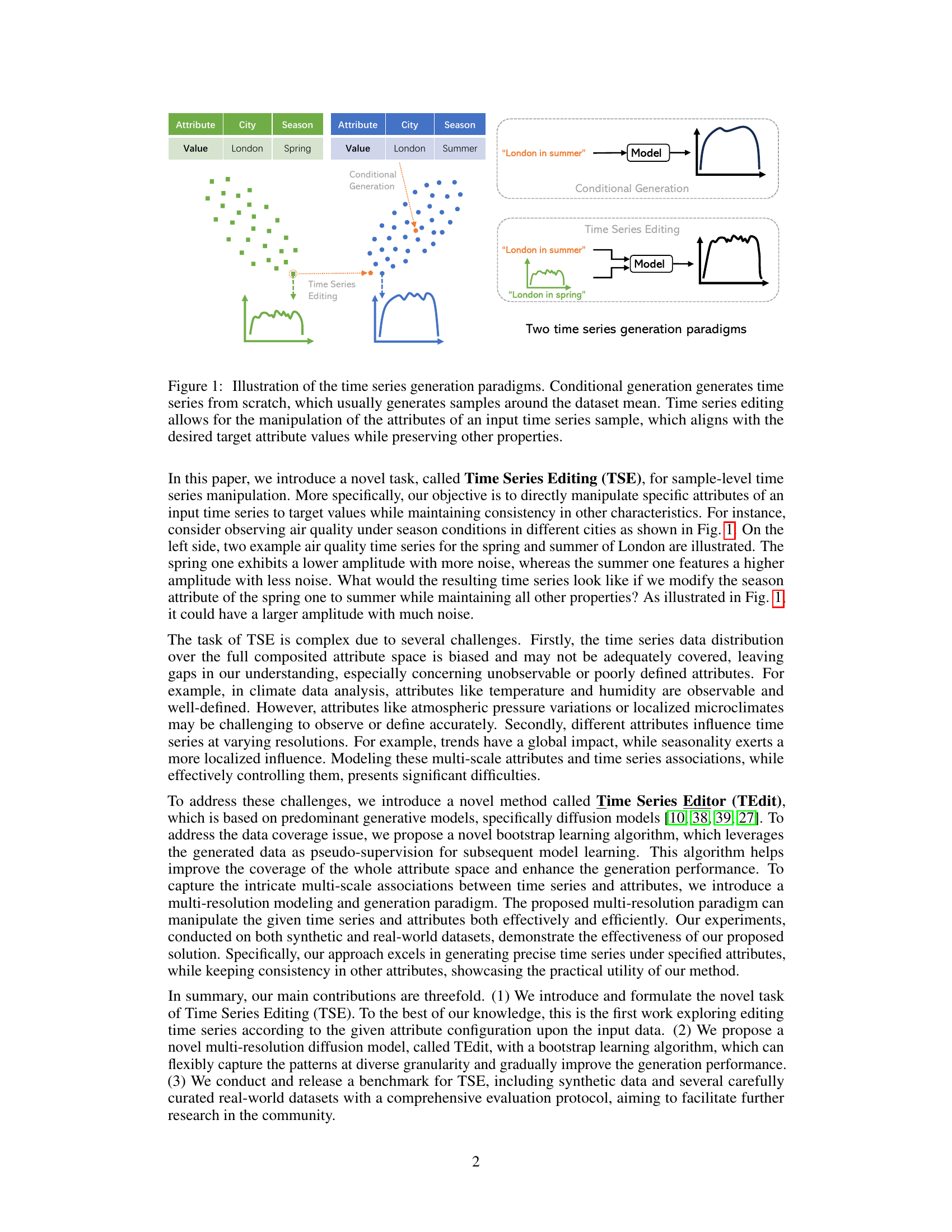
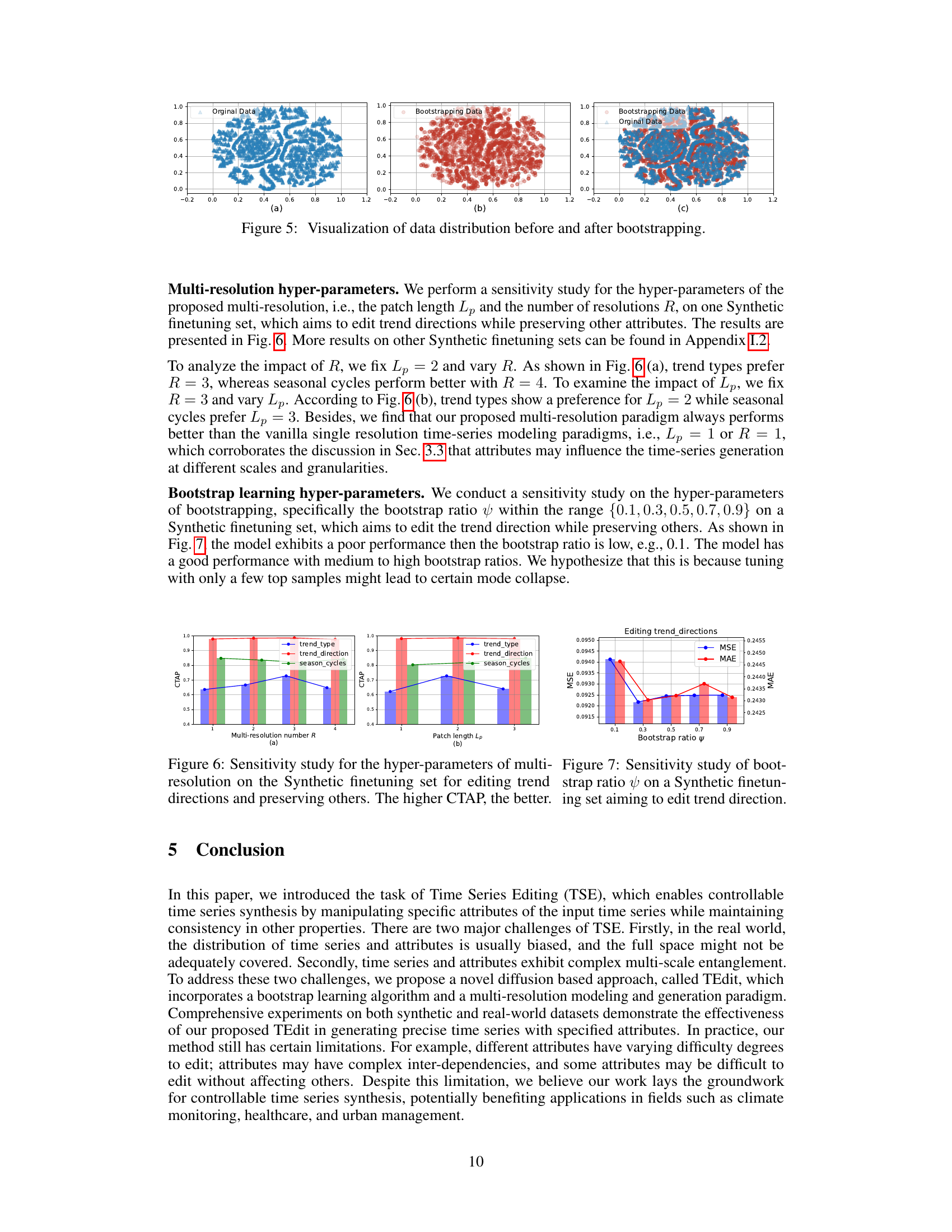
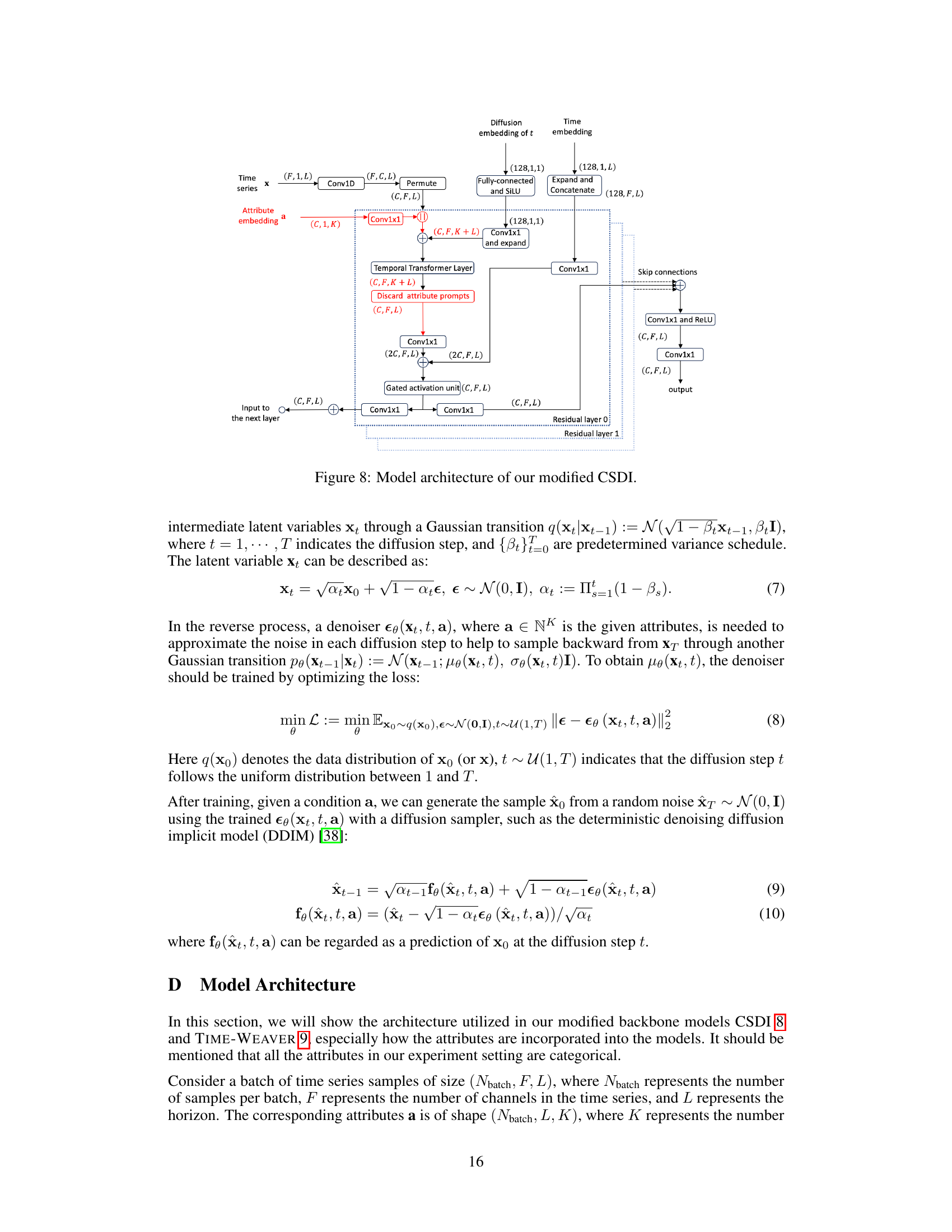
🔼 This figure illustrates the two-stage process of the Time Series Editor (TEdit) model. The upper part shows how the model encodes the source time series and its attributes into a latent representation using a forward diffusion process, then decodes the latent representation with the target attributes to generate the edited time series using a reverse diffusion process. The lower part shows the bootstrap learning process, where the generated time series is self-scored by editing it back to the original time series to improve the model’s performance.
read the caption
Figure 2: Illustration of the editing function Φθ (upper) and the process of self-scoring the generated for bootstrap learning (lower). Upper: Φθ(xsrc, asrc, atgt) first encodes the source (xsrc, asrc) into the latent viable x via the forward DDIM Eq.(4), and then decodes x with the target attributes atgt: (xsrc, atgt) into x tgt via the reverse DDIM in Eq.(5). See Sec. 3.2 for more details. Lower: during bootstrap learning, we use Φθ to self-score the generated x tgt by editing it back to xsrc, and obtain the score s = MSE(xsrc, xsrc), see Sec. 3.4 for more details.

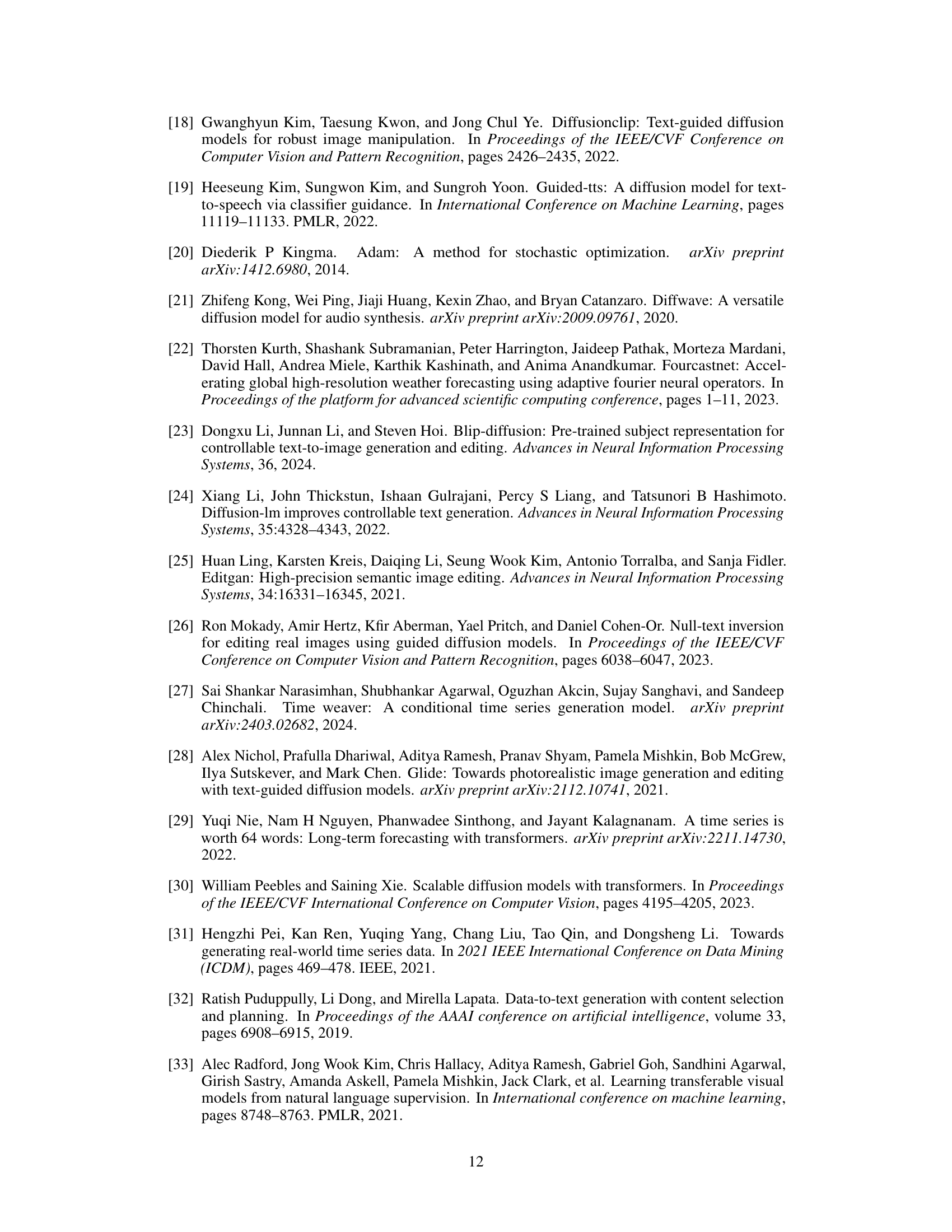
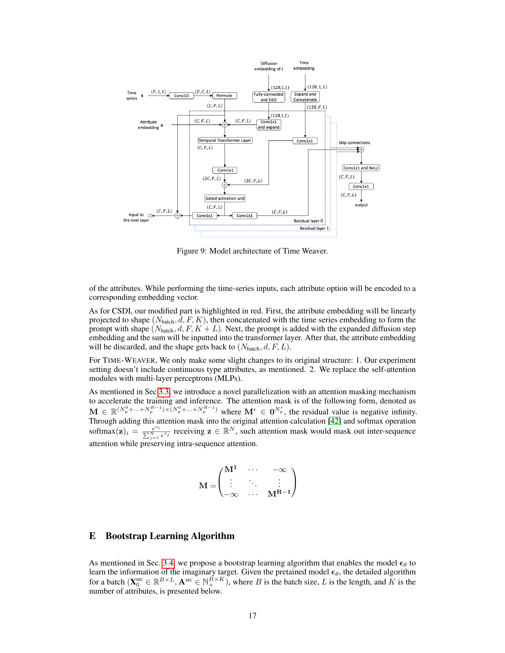
🔼 This figure shows the architecture of the multi-resolution noise estimator, a key component of the TEdit model. The input noisy time series is first patchified into multiple sequences of different resolutions. These sequences, along with input attributes and diffusion steps, are processed by a multi-patch encoder and a multi-patch decoder. A processing module captures multi-scale associations between time series and attributes. Finally, a multi-layer perceptron (MLP) combines the estimations from different resolutions to produce the final estimated noise.
read the caption
Figure 3: Architecture of the proposed multi-resolution noise estimator εθ. We illustrate with R = 3 patching schema, patch length Lp = 2−1,r ∈ {1, ..., R} and the input length L = 8. N = [L/Lp]r is the patch number. D is the embedding size. Please refer to Sec. 3.3 for details.

🔼 This figure compares two time series generation methods: conditional generation and time series editing. Conditional generation synthesizes time series from scratch, resulting in samples clustered around the data mean, lacking fine-grained control. In contrast, time series editing modifies an existing time series sample to match specified attribute values while preserving other characteristics. This allows for more precise control and aligns better with ‘what-if’ scenarios in time series analysis.
read the caption
Figure 1: Illustration of the time series generation paradigms. Conditional generation generates time series from scratch, which usually generates samples around the dataset mean. Time series editing allows for the manipulation of the attributes of an input time series sample, which aligns with the desired target attribute values while preserving other properties.

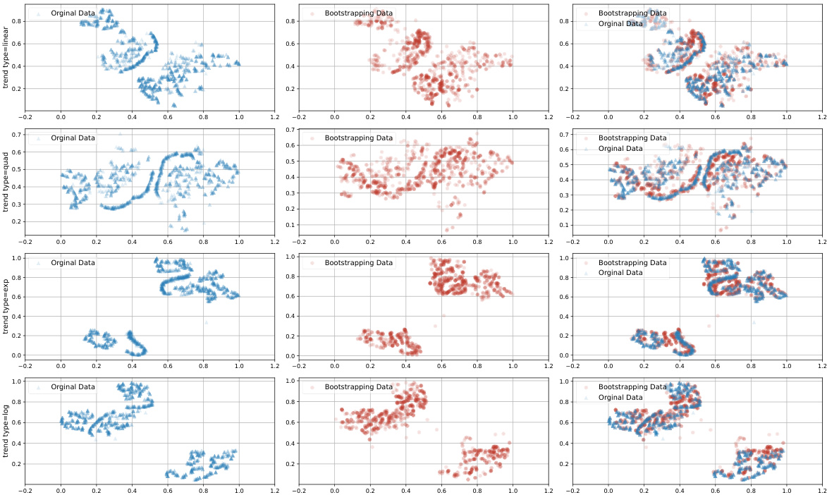
🔼 This figure visualizes the impact of bootstrapping on the distribution of data in the attribute space. It uses t-SNE to reduce the dimensionality of the data and shows the distribution before bootstrapping (original data), the distribution after bootstrapping (bootstrapping data), and a combined visualization of both. The visualizations help illustrate how bootstrapping expands the coverage of the attribute space by generating samples in previously under-represented regions.
read the caption
Figure 5: Visualization of data distribution before and after bootstrapping.

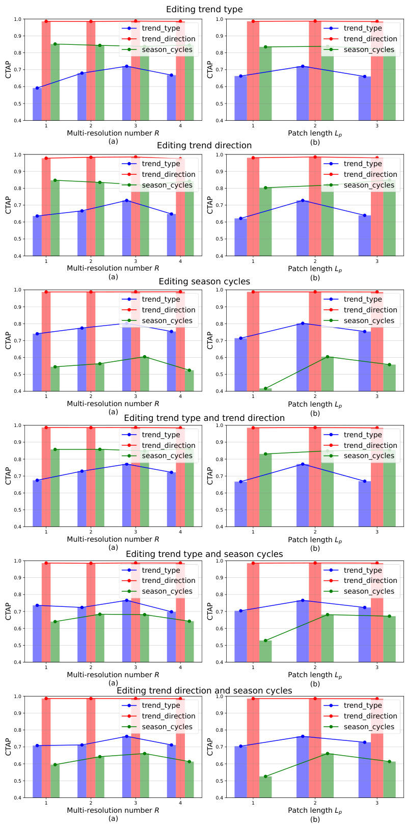
🔼 The figure shows the impact of multi-resolution parameters (number of resolutions R and patch length Lp) on different attributes in 6 synthetic subsets. Each subset involves editing a different combination of attributes: trend type, trend direction, and season cycles. The results (CTAP scores) are presented as bar charts, showing the performance for each attribute across different resolutions and patch lengths. This visualization demonstrates that different attributes have varying sensitivities to different multi-resolution configurations.
read the caption
Figure 11: The impact of multi-resolution on 6 Synthetic subsets.

🔼 The figure depicts the architecture of the multi-resolution noise estimator used in the Time Series Editor (TEdit) model. It shows how the input noisy time series is processed through multiple resolutions using patching, encoding, processing, and decoding modules to estimate the noise. The different resolutions allow the model to capture multi-scale relationships between the time series and attributes.
read the caption
Figure 3: Architecture of the proposed multi-resolution noise estimator εθ. We illustrate with R = 3 patching schema, patch length Lp = 2−1,r ∈ {1, ..., R} and the input length L = 8. N = [L/Lp]r is the patch number. D is the embedding size. Please refer to Sec. 3.3 for details.

🔼 This figure shows the architecture of the multi-resolution noise estimator, a key component of the TEdit model. It uses a multi-patch encoder and decoder to process time series data at multiple resolutions, capturing multi-scale relationships between the time series and its attributes. The input is a noisy time series, attributes, and the diffusion step. The output is the estimated noise at different resolutions. These are then combined using a multi-layer perceptron (MLP).
read the caption
Figure 3: Architecture of the proposed multi-resolution noise estimator εθ. We illustrate with R = 3 patching schema, patch length Lp = 2−1,r ∈ {1, ..., R} and the input length L = 8. N = [L/Lp]r is the patch number. D is the embedding size. Please refer to Sec. 3.3 for details.
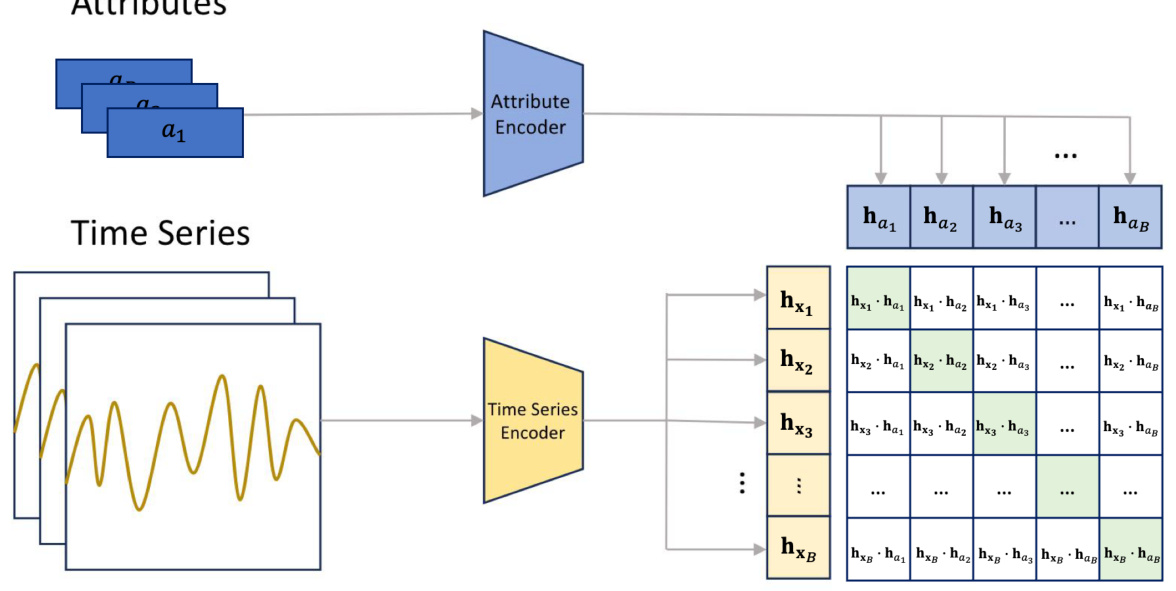
🔼 This figure illustrates the architecture of the Contrastive Time series Attribute Pretraining (CTAP) model. The model takes pairs of time series and their corresponding attributes as input. It uses separate encoders for time series and attributes to extract their embeddings. The model then calculates pairwise similarities between the time series and attribute embeddings and is trained to distinguish positive (matching) and negative (non-matching) pairs. This training process helps the model learn the alignment between time series and attributes, which is useful for evaluating the quality of time series editing.
read the caption
Figure 10: Illustration of the CTAP model for the given pairs of time series X = {x}B=1 and attributes A = {ai}B=1, where B is the batch size. Here ai = ak = a[k], k ∈ {1, ..., K} is the k-th attribute of the full attribute vector a ∈ NK. We use K separate attribute encoders for K attributes. In the illustration, we only show one attribute and thus drop the attribute index k for clarity. After obtaining embeddings {hx₁}B=1 and {ha₁}B=1, we calculate the the pair-wise similarities between the hx, and ha,. The encoders are trained by distinguishing the positive pairs (green blocks) and negative pairs (white blocks).
🔼 This figure shows the architecture of the multi-resolution noise estimator, a key component of the TEdit model. It illustrates how the model processes the input noisy time series at multiple resolutions (R=3 in this example) to capture multi-scale relationships between time series and attributes. The input time series is divided into patches of varying lengths, processed through encoder and decoder modules, and finally combined to produce the estimated noise. The figure highlights the multi-patch encoder, multi-patch decoder, and processing module, illustrating the multi-resolution paradigm.
read the caption
Figure 3: Architecture of the proposed multi-resolution noise estimator . We illustrate with R = 3 patching schema, patch length Lp = 2−1,r ∈ {1, ..., R} and the input length L = 8. N = [L/Lp] is the patch number. D is the embedding size. Please refer to Sec. 3.3 for details.

🔼 This figure illustrates the two-stage process of the Time Series Editor (TEdit) model. The upper part shows how TEdit modifies the input time series by encoding it into a latent representation and then decoding it with target attributes using the forward and reverse DDIM processes. The lower part illustrates the self-scoring process used in bootstrap learning. This process involves using TEdit to generate a new time series, editing it back to the original input, and comparing it to the original using Mean Squared Error (MSE).
read the caption
Figure 2: Illustration of the editing function Φθ (upper) and the process of self-scoring the generated for bootstrap learning (lower). Upper: Φθ(xsrc, asrc, atgt) first encodes the source (xsrc, asrc) into the latent viable x via the forward DDIM Eq.(4), and then decodes x with the target attributes atgt: (xsrc, atgt) into xtgt via the reverse DDIM in Eq.(5). See Sec. 3.2 for more details. Lower: during bootstrap learning, we use Φθ to self-score the generated xtgt by editing xtgt back to xsrc, and obtain the score s = MSE(xsrc, xsrc), see Sec. 3.4 for more details.

🔼 This figure illustrates two different approaches to generating time series data: conditional generation and time series editing. Conditional generation starts from scratch, creating entirely new time series based on learned data distributions. The generated samples tend to cluster around the average characteristics of the training data. In contrast, time series editing takes an existing time series as input and modifies specific attributes (e.g., changing the season from spring to summer) while preserving other properties. This allows for a more targeted and controllable synthesis process, enabling the manipulation of existing samples rather than generating entirely new ones.
read the caption
Figure 1: Illustration of the time series generation paradigms. Conditional generation generates time series from scratch, which usually generates samples around the dataset mean. Time series editing allows for the manipulation of the attributes of an input time series sample, which aligns with the desired target attribute values while preserving other properties.
🔼 This figure illustrates the Time Series Editor (TEdit) framework. The upper panel shows the two-stage editing process: forward diffusion to encode the source time series and attributes into a latent variable, followed by reverse diffusion to decode the latent variable with target attributes, generating the edited time series. The lower panel illustrates the self-scoring mechanism used in bootstrap learning, where the generated time series is edited back to the original using the same process, and the mean squared error (MSE) between the original and edited time series serves as the score for evaluating the generated time series.
read the caption
Figure 2: Illustration of the editing function Φθ (upper) and the process of self-scoring the generated for bootstrap learning (lower). Upper: Ф(xrc, asrc, atgt) first encodes the source (x, asrc) into the latent viable x via the forward DDIM Eq.(4), and then decodes x with the target attributes atgt: (xsrc, atgt) into via the reverse DDIM in Eq.(5). See Sec. 3.2 for more details. Lower: during bootstrap learning, we use Φe to self-score the generated by editing back to xsrc, and obtain the score s = MSE(, xsrc), see Sec. 3.4 for more details.

🔼 This figure shows the architecture of the multi-resolution noise estimator used in the Time Series Editor (TEdit) model. It illustrates how the model processes the input time series at multiple resolutions (R=3 in this example) using patches of varying lengths (Lp). Each resolution’s patches are encoded and processed separately, capturing different levels of detail in the time series data. The processed information is then combined to produce a final noise estimation which is used in the diffusion process.
read the caption
Figure 3: Architecture of the proposed multi-resolution noise estimator ϵθ. We illustrate with R = 3 patching schema, patch length Lp = 2−1,r ∈ {1, ..., R} and the input length L = 8. N = [L/Lp] is the patch number. D is the embedding size. Please refer to Sec. 3.3 for details.

🔼 This figure visualizes the effect of bootstrapping on the data distribution using t-SNE. It compares the distribution of the original data, the generated data after training with only the original data, and the distribution of both the original and the generated data combined. The visualization aims to show how the bootstrapping process improves the data coverage and fills in gaps in the attribute space. The improved coverage is expected to improve the model’s ability to edit time series attributes.
read the caption
Figure 5: Visualization of data distribution before and after bootstrapping.
More on tables

🔼 This table presents the results of ablation studies conducted on three datasets (Synthetic, Air, and Motor) to analyze the impact of different components of the proposed Time Series Editor (TEdit) model. Specifically, it examines the effects of using ground truth data (GT), the bootstrap learning algorithm (BS), and the multi-resolution approach (MR) on the model’s performance in editing and preserving time series attributes. The table shows average metrics across all finetuning sets for each dataset, broken down by whether the attributes were edited or preserved. This allows for a clear comparison of the impact of each component on the model’s overall performance and attribute-specific performance.
read the caption
Table 2: Ablation studies on the Synthetic, Air and Motor datasets. GT, BS and MR refer to Ground Truth source and target pairs, BootStrap and Multi-Resolution. Results are averaged over all finetuning sets. “Edited” and “Preserved” are the average results of all edited and preserved attributes.
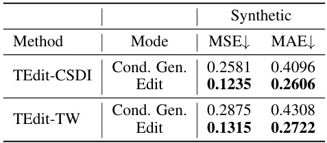
🔼 This table presents the average performance of different methods (CSDI, Time Weaver, TEdit-CSDI, TEdit-TW) across three datasets (Synthetic, Air, Motor) for both edited and preserved attributes. The metrics used are RaTS (Log Ratio of Target-to-Source probability) and CTAP (Contrastive Time series Attribute Pretraing) score, reflecting the ability to edit and preserve attributes respectively. Lower MSE and MAE values on the Synthetic dataset indicate better performance in terms of numerical accuracy. The table summarizes results from multiple finetuning sets, providing a comprehensive evaluation of the methods’ performance.
read the caption
Table 1: Averaged performance over all finetuning sets for Synthetic (left), Air (middle), and Motor (right). 'Edited' and 'Preserved' are the average results of all edited and preserved attributes.

🔼 This table presents the average performance of different methods (CSDI, Time Weaver, TEdit-CSDI, and TEdit-TW) across three datasets (Synthetic, Air, and Motor). The performance is measured by metrics such as RaTS, CTAP, MSE, and MAE, separately for edited and preserved attributes. The results demonstrate the superiority of the TEdit models in both editing and preserving attributes in the time series.
read the caption
Table 1: Averaged performance over all finetuning sets for Synthetic (left), Air (middle), and Motor (right). 'Edited' and 'Preserved' are the average results of all edited and preserved attributes.

🔼 This table presents the averaged performance of different methods (CSDI, Time Weaver, TEdit-CSDI, TEdit-TW) on three datasets (Synthetic, Air, Motor) across all finetuning sets. The performance is measured using RaTS, CTAP, MSE, and MAE scores, separated for ’edited’ and ‘preserved’ attributes, indicating the model’s ability to modify specified attributes while maintaining other characteristics. Higher RaTS and CTAP values generally indicate better performance.
read the caption
Table 1: Averaged performance over all finetuning sets for Synthetic (left), Air (middle), and Motor (right). 'Edited' and 'Preserved' are the average results of all edited and preserved attributes.

🔼 This table presents the average performance of different methods across three datasets (Synthetic, Air, and Motor) for both edited and preserved attributes. The metrics used include RaTS (Log Ratio of Target-to-Source probability), CTAP score (Contrastive Time series Attribute Pretraining), MSE (Mean Squared Error), and MAE (Mean Absolute Error). The results show the performance of the proposed TEdit method in comparison to baseline methods (CSDI and Time Weaver).
read the caption
Table 1: Averaged performance over all finetuning sets for Synthetic (left), Air (middle), and Motor (right). 'Edited' and 'Preserved' are the average results of all edited and preserved attributes.

🔼 This table shows the top 1 and top 2 classification accuracy of the CTAP model on different datasets. The CTAP model is used to measure the alignment between the generated time series and real-world time series associated with given attribute values. Higher accuracy indicates better alignment. The table includes results for synthetic data (trend types, trend directions, season cycles) and real-world datasets (Air Quality: city and season; Motor Imagery: channel ID and imagined movement).
read the caption
Table 7: The performance of CTAP models on different datasets. We report the top-1 and top-2 classification accuracy for each attribute on the test sets of the pertaining dataset.
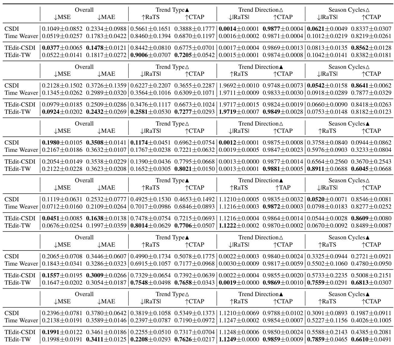
🔼 This table presents the average performance of different methods (CSDI, Time Weaver, TEdit-CSDI, and TEdit-TW) across three datasets (Synthetic, Air, and Motor) for both edited and preserved attributes. The performance is measured using RaTS (Ratio of Target-to-Source), CTAP (Contrastive Time series Attribute Pretraining) score, MSE (Mean Squared Error), and MAE (Mean Absolute Error). The results show that TEdit outperforms the baselines in most metrics, demonstrating its effectiveness in editing time series while preserving other properties.
read the caption
Table 1: Averaged performance over all finetuning sets for Synthetic (left), Air (middle), and Motor (right). 'Edited' and 'Preserved' are the average results of all edited and preserved attributes.

🔼 This table presents the average performance results across all finetuning sets for three datasets: Synthetic, Air, and Motor. For each dataset, it shows the performance metrics for both the edited and preserved attributes. The metrics used include RaTS (Log Ratio of Target-to-Source probability), CTAP (Contrastive Time series Attribute Pretraing) score, MSE (Mean Squared Error), and MAE (Mean Absolute Error). Higher RaTS and CTAP scores indicate better performance for edited attributes, while lower |RaTS| and higher CTAP scores indicate better performance for preserved attributes. MSE and MAE are only reported for the Synthetic dataset.
read the caption
Table 1: Averaged performance over all finetuning sets for Synthetic (left), Air (middle), and Motor (right). 'Edited' and 'Preserved' are the average results of all edited and preserved attributes.
Full paper#
