↗ OpenReview ↗ NeurIPS Homepage ↗ Chat
TL;DR#
Machine learning models often inherit biases present in training data, significantly impacting their performance across different groups. Existing research primarily focuses on the initial and final stages of learning, neglecting the crucial transient dynamics where bias evolves. This study addresses this gap by investigating bias’s dynamic behavior throughout training using a teacher-student framework and Gaussian mixture models to represent diverse data sub-populations.
The research employs high-dimensional analysis, deriving an analytical solution for the stochastic gradient descent dynamics. This analysis reveals the evolution of bias across three distinct phases: an initial phase dominated by class imbalance, an intermediate phase driven by sample saliency, and a final phase determined by sub-population representation. The findings are empirically validated using deeper networks on various datasets, demonstrating the prevalence and complexity of this dynamic bias across different training scenarios. This work significantly contributes to a deeper understanding of bias formation and provides crucial insights for developing more effective bias mitigation techniques.
Key Takeaways#
Why does it matter?#
This paper is crucial for researchers working on fairness and robustness in machine learning. It provides a novel theoretical framework for understanding the transient dynamics of bias, which is often overlooked in existing research. This framework offers new avenues for developing effective bias mitigation strategies and prompts further studies on the evolution of biases at different stages of training.
Visual Insights#

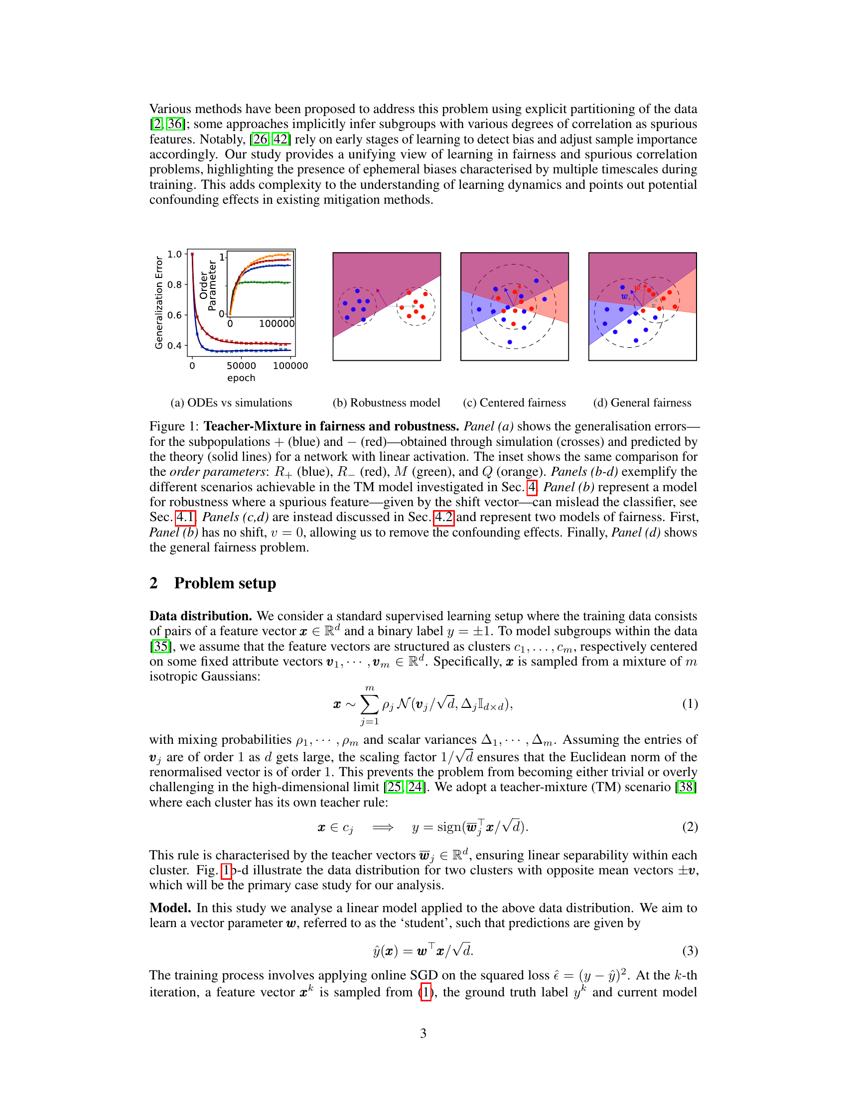
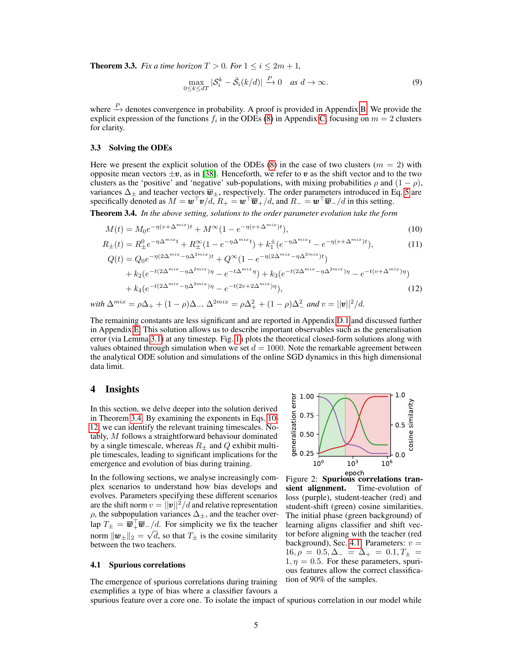
This figure demonstrates the generalization error for different subpopulations in a teacher-mixture model. Panel (a) compares simulated and theoretical results using a linear activation network, showing a good fit. The inset shows a comparison for the order parameters. Panels (b) through (d) showcase various scenarios achievable using the teacher-mixture model, relating to robustness and fairness.
In-depth insights#
Bias Dynamics#
The study of bias dynamics in machine learning reveals a complex interplay of factors influencing how biases evolve during training. Initial phases often show a classifier’s sensitivity to class imbalances within subpopulations, leading to an initial bias towards more represented groups. Intermediate stages highlight a shift towards the saliency of sample features, where the classifier focuses on features that are more readily apparent, regardless of their predictive power. The final stage emphasizes the dominance of relative subpopulation representation in the model, solidifying biases through numerical preponderance over other data characteristics. High-dimensional analysis provides an analytical framework to understand this evolution, proving the accuracy of ODEs in predicting bias dynamics in higher dimensions. Empirical validation through synthetic and real datasets supports these theoretical findings, further reinforcing the significance of the observed temporal dynamics of bias formation in machine learning systems. This understanding is crucial in developing effective bias mitigation strategies.
High-D Analysis#
The heading ‘High-D Analysis’ suggests a focus on the theoretical properties of high-dimensional data and algorithms. The authors likely leverage tools from statistical physics or random matrix theory to analyze the behavior of the model in high dimensions. This approach is crucial because the behavior of machine learning models often changes dramatically as the dimensionality of the data increases. Instead of relying on empirical observations alone, this high-dimensional analysis provides a rigorous mathematical framework for understanding the dynamics of bias in stochastic gradient descent. A key strength of such an approach is the ability to derive closed-form expressions or approximate solutions for model behavior, offering insights unavailable through solely experimental means. The high-dimensional setting allows the authors to make simplifying assumptions that lead to tractable analytical results, such as the convergence of stochastic dynamics to deterministic ordinary differential equations. The analytical solutions derived in this section can be used to validate and complement the experimental results, providing further confidence in the observed phenomena. Overall, the ‘High-D Analysis’ section likely plays a pivotal role in establishing a strong theoretical foundation for the paper’s findings.
SGD Dynamics#
The study delves into the dynamics of Stochastic Gradient Descent (SGD) optimization, focusing on how bias evolves during the training process. It uses a teacher-student framework with Gaussian mixture models to represent diverse data subpopulations. A key finding is the characterization of bias evolution into three distinct phases, each influenced by different data properties: initial imbalance, sample saliency, and relative representation. This reveals a non-monotonic behavior of bias, challenging the conventional focus on only initial or final states. The analysis leverages a high-dimensional limit, enabling analytical solutions for the dynamics, which are then validated empirically with deeper networks on real datasets. This provides valuable insights into transient learning regimes and highlights the dynamic interplay between various factors like data heterogeneity, spurious features, and class imbalance in shaping bias. The implications are significant for fairness and robustness, showing how to understand and potentially mitigate bias through a deeper understanding of its evolution over time.
Bias Mitigation#
The concept of bias mitigation in machine learning is crucial, as models trained on biased data often perpetuate or amplify those biases. This paper delves into the dynamics of bias in stochastic gradient descent (SGD) training, offering valuable insights for developing effective mitigation strategies. The analysis reveals how different properties of subpopulations influence bias at different timescales, highlighting the non-monotonic nature of bias evolution during training. This understanding is crucial, as it moves beyond simplistic views of bias as merely an initial or final state. A three-phase learning process is identified where bias is influenced by factors such as class imbalance, data representation, and spurious correlations. The research emphasizes the importance of considering this transient bias evolution for effective mitigation strategies. The analytical framework developed is validated using experiments on synthetic and real datasets, showing promise in guiding the development of targeted and temporally-aware bias mitigation techniques. Ultimately, this work underscores the need for going beyond asymptotic analysis when considering bias and calls for the development of methods that account for the complex temporal dynamics of bias in machine learning.
Future Work#
Future research directions stemming from this work could explore several promising avenues. Extending the theoretical analysis to more complex model architectures (beyond linear classifiers and shallow networks) is crucial to assess the generalizability of the findings. Investigating the impact of different activation functions, network depths, and training algorithms on bias dynamics would provide valuable insights. Developing bias mitigation strategies directly informed by the identified transient dynamics is another key area. This could involve designing adaptive learning rates or regularization techniques that specifically target the critical phases of bias formation. Empirical validation on a wider array of real-world datasets, encompassing diverse domains and demographic groups, is necessary to further test the robustness and practical applicability of the proposed theoretical framework. Finally, a deeper investigation into the interplay between bias and other ML phenomena, like generalization and spurious correlations, could yield a more holistic understanding of how bias manifests in the learning process. This integrated understanding is critical to creating effective and robust strategies for building fair and equitable machine learning systems.
More visual insights#
More on figures

This figure shows the generalization error of a linear classifier trained using SGD on a dataset generated from a teacher-mixture model. Panel (a) compares the theoretical predictions of generalization error with the results from simulations, showing a good match. The inset in panel (a) compares the order parameters from theory and simulations. Panels (b-d) demonstrate different scenarios (robustness and fairness) achievable with the teacher-mixture model.

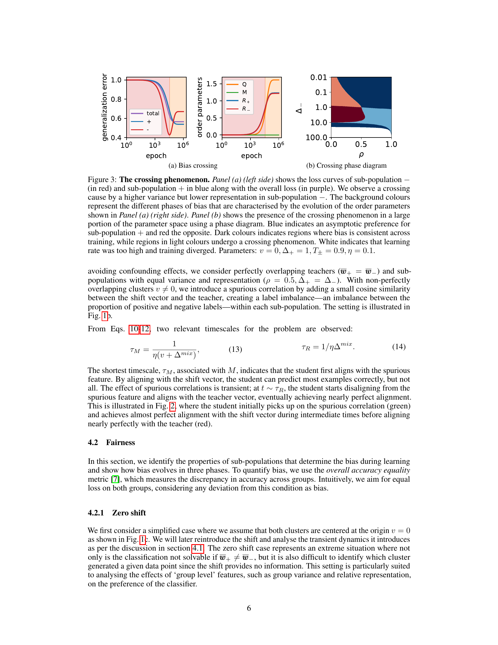
This figure demonstrates the ‘crossing phenomenon’ where the loss curves of two sub-populations intersect during training. Panel (a) shows the loss curves for sub-population + (blue) and sub-population – (red), along with the total loss (purple). The crossing is caused by sub-population – having higher variance but lower representation. The right panel shows the order parameters over time illustrating the different bias phases. Panel (b) presents a phase diagram highlighting the parameter regions where the crossing phenomenon occurs. The color scheme in the phase diagram indicates the asymptotic preference of the classifier (blue for sub-population +, red for sub-population –). Dark colors show consistent bias, light colors show a bias crossing, and white represents divergence due to high learning rates.

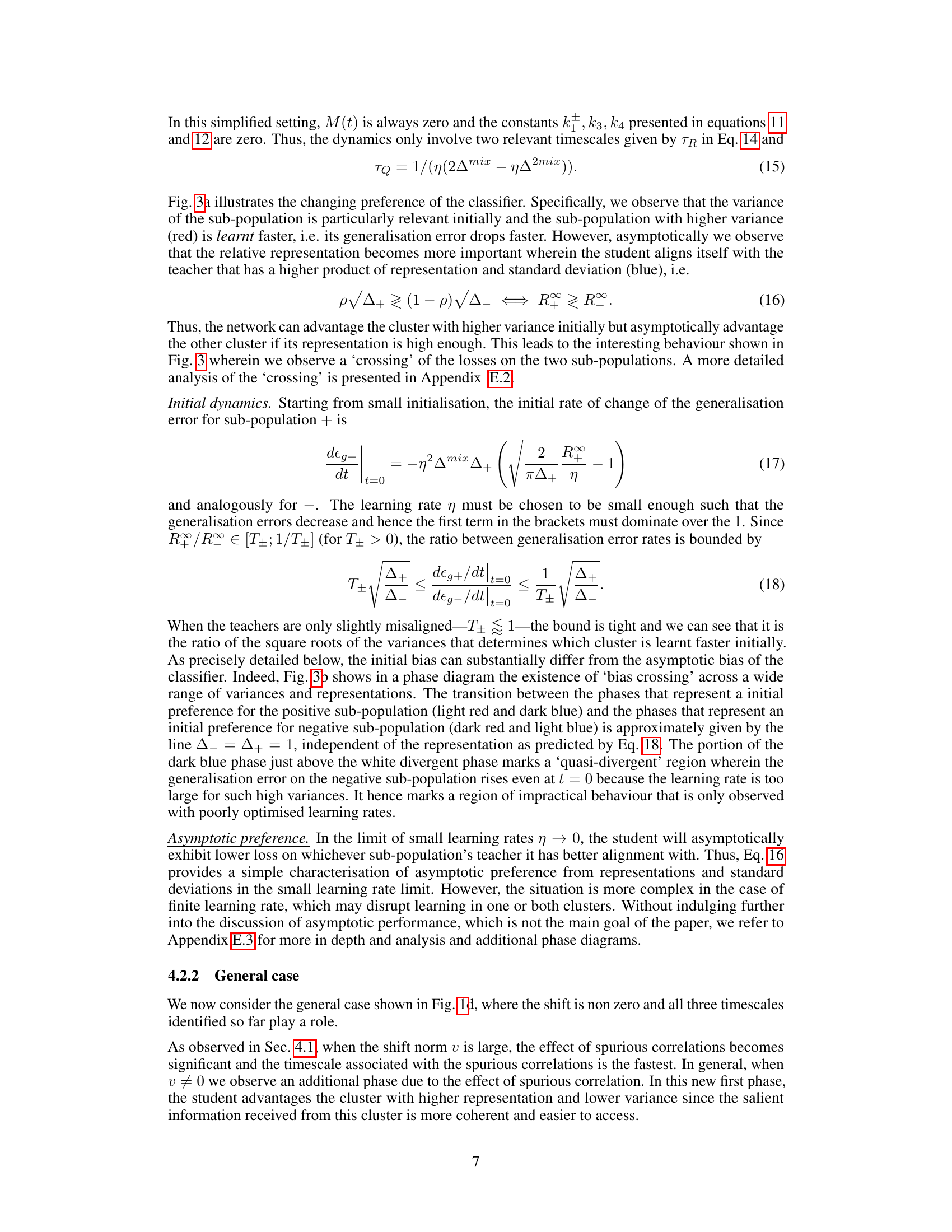
This figure shows the phenomenon of bias crossing in which the loss curves for different sub-populations intersect during training, highlighting the non-monotonic nature of bias in this setting. The left panel displays the loss curves for the positive and negative sub-populations and their average, illustrating the crossing behavior. The right panel shows the evolution of multiple order parameters which help to explain this behavior, showing three distinct learning phases. Key parameters determining this behavior are also provided.
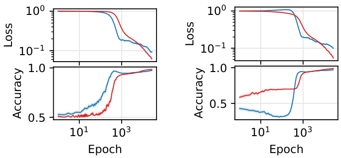
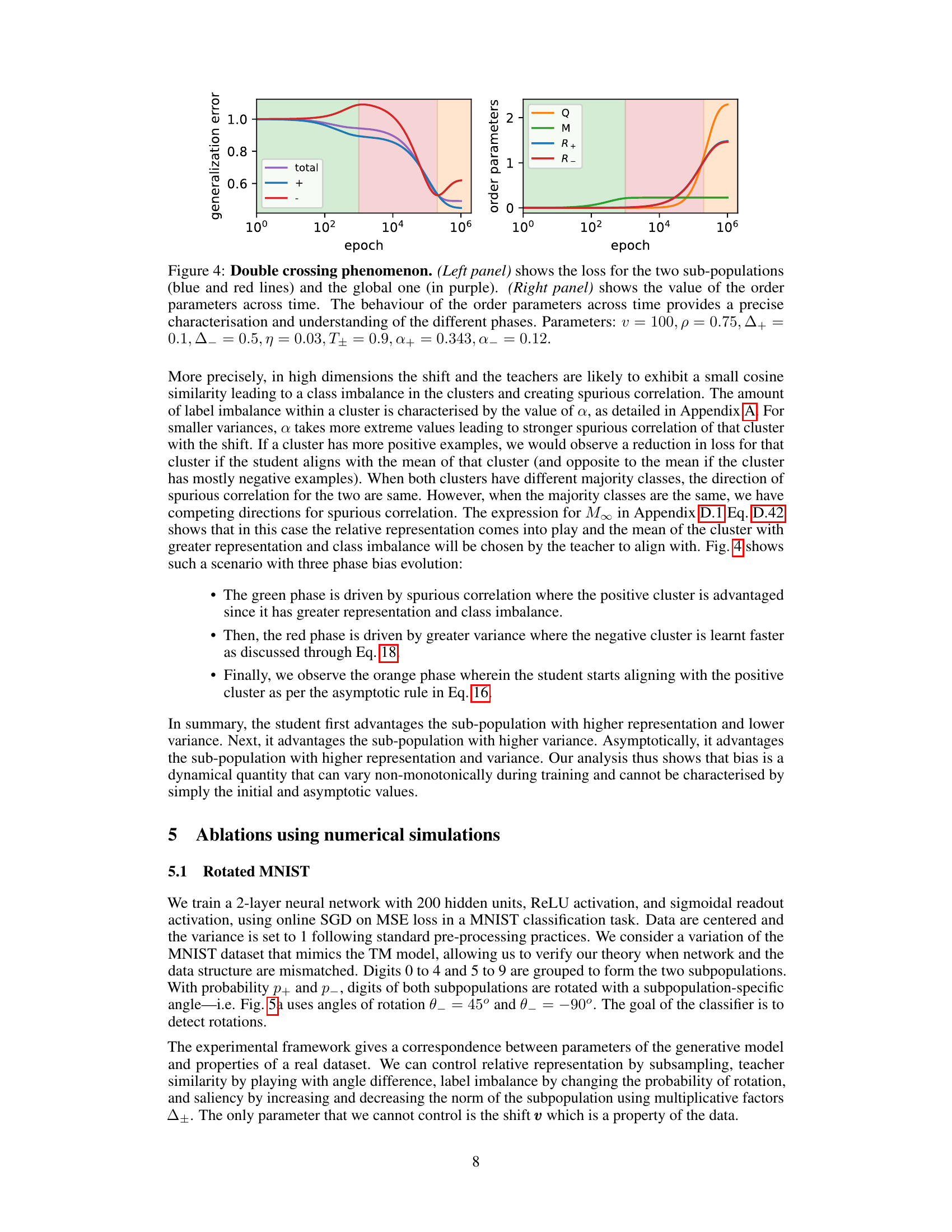
This figure presents numerical simulation results on the MNIST dataset using a 2-layer neural network. It demonstrates the evolution of test loss and accuracy for two subpopulations (+) and (-) over multiple training epochs. Three panels showcase different scenarios: a single crossing phenomenon, a double crossing phenomenon (introducing a label imbalance), and the effect of varying variance while keeping one variance constant. Each panel shows the average and standard deviation over 100 simulations, illustrating the robustness of the observed phenomena.

This figure presents the results of numerical simulations conducted on the MNIST dataset to validate the theoretical findings. It showcases three scenarios: a single crossing phenomenon, a double crossing phenomenon, and an analysis of the impact of changing the variance of one subpopulation while keeping the variance of the other constant. Each panel displays the test loss and accuracy for two subpopulations over multiple epochs. The results demonstrate the presence of multiple time scales in the bias dynamics and how they lead to non-monotonic behavior of the classifier.

This figure shows the results of numerical simulations on the MNIST dataset using a variation of the Teacher-Mixture model. The top row shows test loss, and the bottom row shows test accuracy, for two sub-populations (+ in blue, - in red). Panel (a) demonstrates a single crossing phenomenon where the loss curves for the two subpopulations intersect during training. Panel (b) shows a double crossing, indicating a more complex bias evolution with multiple timescale dynamics. Panel (c) explores how the initial bias in learning depends on the variances of the subpopulations.
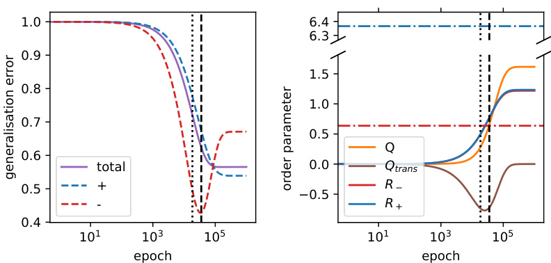
The left panel of the figure shows the loss curves for the negative (red) and positive (blue) sub-populations, as well as the overall loss (purple). The crossing of the loss curves is highlighted, with the dashed and dotted vertical lines indicating important timescales. The right panel displays the dynamics of order parameters over time, illustrating the three phases of bias.
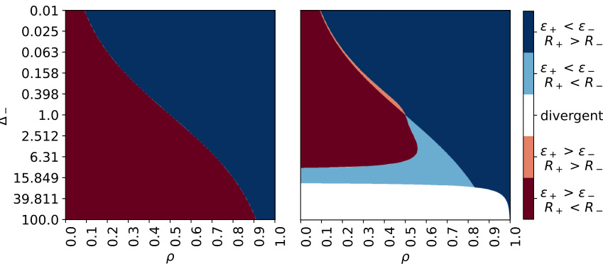
This figure shows the loss curves and phase diagrams demonstrating the ‘crossing phenomenon.’ The left panel shows the loss curves of two sub-populations, highlighting how the sub-population with higher variance initially has faster learning but asymptotically the sub-population with higher representation (product of representation and variance) takes over. The right panel shows a phase diagram illustrating the prevalence of the crossing phenomenon across different parameter combinations.
This figure shows the loss curves for two sub-populations with different variances and mixing probabilities, along with the overall loss. Panel (a) demonstrates a ‘crossing’ phenomenon where initially the higher variance sub-population has lower loss, but asymptotically the sub-population with higher representation (and product of variance and representation) dominates. Panel (b) displays a phase diagram illustrating the regions in parameter space exhibiting this crossing behavior.

This figure demonstrates the generalization errors for two sub-populations in a teacher-student model using a linear activation function. Panel (a) compares the theoretical predictions with simulation results, highlighting the accuracy of the theoretical model. The inset shows the same comparison for order parameters R+, R-, M, and Q. Panels (b) through (d) illustrate different scenarios in the Teacher-Mixture (TM) model. Panel (b) showcases a robustness model where a spurious feature leads to misclassification; Panels (c) and (d) present two fairness models, with Panel (c) being a simplified case and Panel (d) showing the general fairness problem. The figure illustrates the TM model’s ability to represent different fairness and robustness scenarios.

This figure shows the results of numerical simulations on the MNIST dataset using a rotated version of the dataset to mimic the teacher-mixture model presented in the paper. It demonstrates three key phenomena related to bias evolution during training: (a) a single crossing of the loss curves for two subpopulations, (b) a double crossing due to label imbalance, and (c) the impact of changing the variance of one subpopulation while keeping the other constant. The results validate the theoretical analysis by showing the predicted multi-phase behavior in a more realistic setting.

This figure shows the generalization errors for different sub-populations and how the theoretical predictions match the simulation results for a linear activation network. The inset shows a comparison of order parameters. It also exemplifies different fairness and robustness models using the teacher-mixture framework, showing how spurious features and heterogeneous data can affect the classifier’s behavior during learning.

This figure shows the generalization errors for two subpopulations in a teacher-student learning model. Panel (a) compares the theoretical predictions with simulation results for a linear classifier. Panels (b) through (d) illustrate different scenarios for robustness and fairness, demonstrating how the model can represent various bias situations.
Full paper#
