↗ OpenReview ↗ NeurIPS Homepage ↗ Chat
TL;DR#
Sparse ridge regression is a vital technique in machine learning, yet existing methods often lack speed or accuracy. The OKRidge algorithm emerged as a promising solution, but its theoretical foundation needed improvement. This paper tackles this limitation.
The researchers tackled this by recasting the OKRidge algorithm’s error estimation as a primary optimization problem and employing the Convex Gaussian min-max theorem to simplify it. This allowed them to conduct a theoretical error analysis, proving the algorithm’s effectiveness and reliability. Their findings were validated experimentally, strengthening the theoretical underpinnings of OKRidge.
Key Takeaways#
Why does it matter?#
This paper is crucial for researchers working on sparse ridge regression, a widely used method in machine learning. It provides a rigorous theoretical analysis of the OKRidge algorithm, offering insights into its reliability and performance. This analysis addresses a critical gap in the understanding of OKRidge, paving the way for improved algorithm design and broader applications.
Visual Insights#
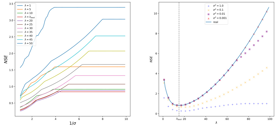
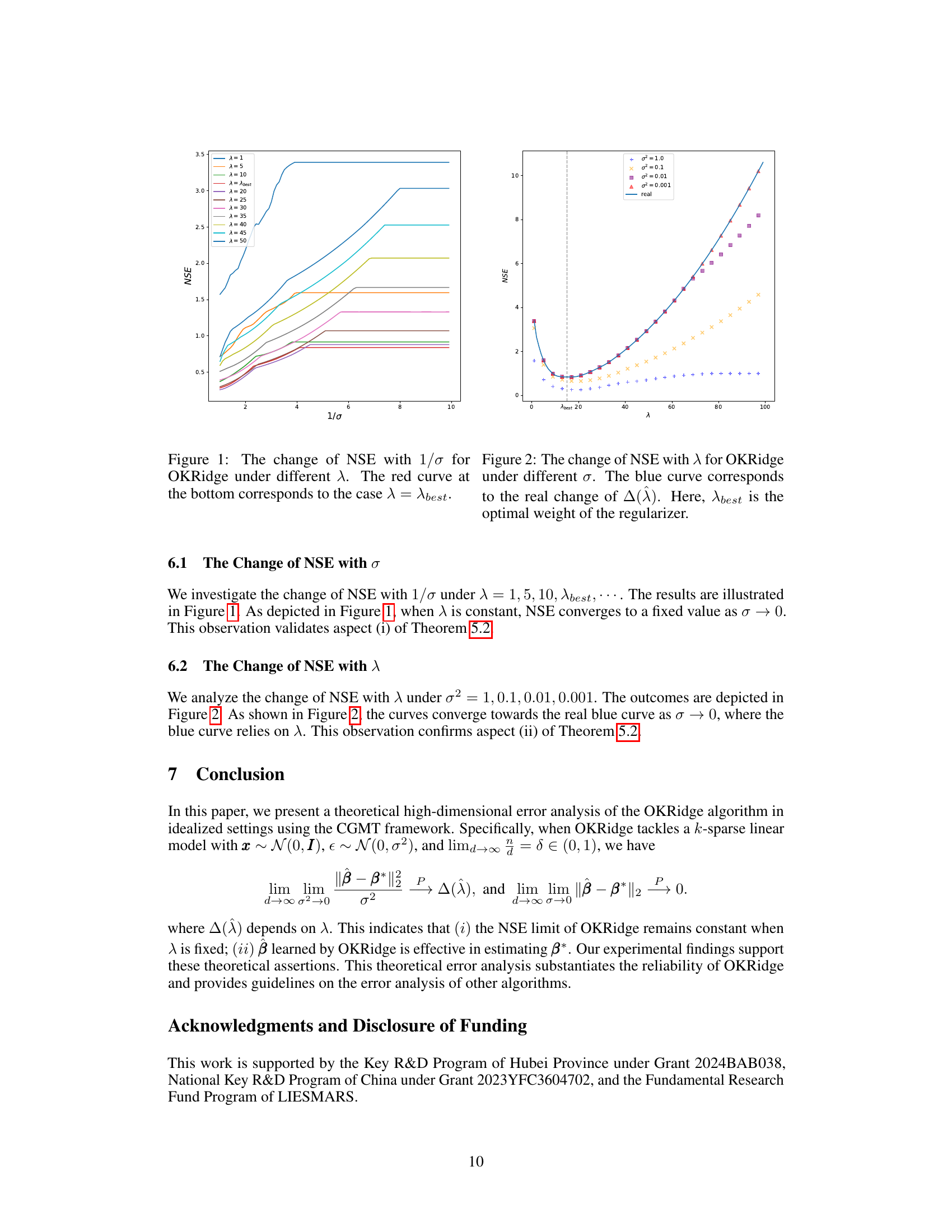
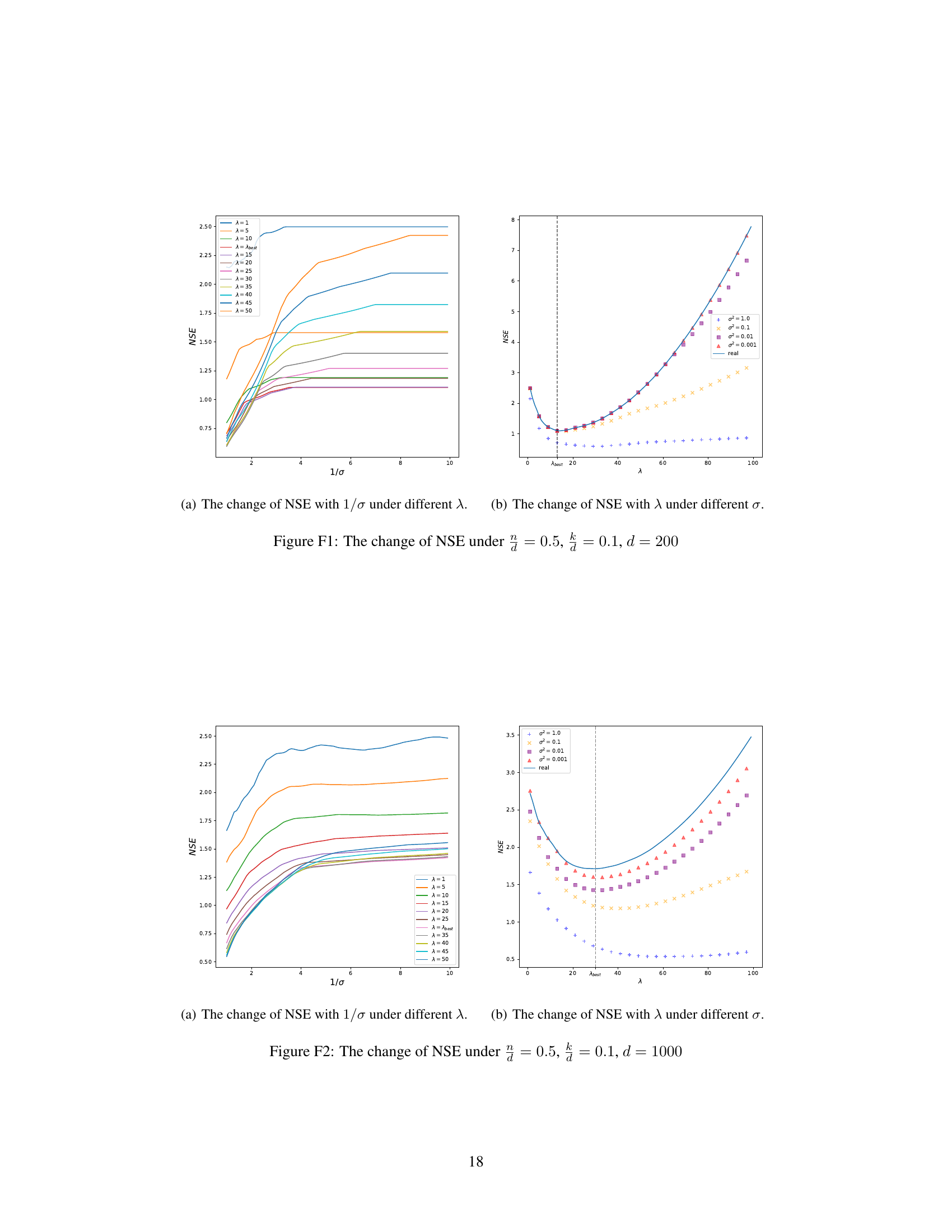
This figure shows the relationship between the Normalized Squared Error (NSE) and the reciprocal of the standard deviation (1/σ) for different values of the regularization parameter λ. Each colored line represents a different λ value, and the lowest line (red) represents the optimal λ value (λbest). As 1/σ increases (meaning the noise level decreases), the NSE generally decreases, indicating improved estimation accuracy. The figure supports the observation that, when λ is constant, the NSE converges to a fixed value as σ → 0.
In-depth insights#
OKRidge Reliability#
The reliability of the OKRidge method for solving sparse ridge regression problems is a crucial aspect of its practical applicability. Theoretical analysis is vital to establish confidence in the method’s performance beyond empirical observations. The paper addresses this by reframing the estimation error as an optimization problem and employing the Convex Gaussian min-max theorem (CGMT) to simplify analysis. This approach provides a theoretical error bound, offering insights into OKRidge’s behavior under various conditions and improving its reliability. Experimental validation corroborates these theoretical findings, strengthening the overall trustworthiness and usefulness of the OKRidge method for sparse ridge regression tasks.
CGMT Error Analysis#
The CGMT (Convex Gaussian Min-max Theorem) error analysis section is crucial for assessing the reliability of the OKRidge algorithm. It leverages CGMT to simplify a complex primary optimization (PO) problem, which directly relates to the estimation error, into a more manageable auxiliary optimization (AO) problem. This simplification is key because the AO problem provides a tractable way to analyze the behavior of the estimation error, specifically the Normalized Squared Error (NSE). The theoretical results derived from the AO problem offer valuable insights into how various factors, such as the regularization parameter (λ) and the noise level (σ), affect the algorithm’s performance. The analysis demonstrates a theoretical guarantee for the reliability of OKRidge by showing that under certain conditions, the error converges to a fixed value determined by λ as the noise approaches zero. This theoretical justification is further supported by the excellent agreement between theoretical predictions and experimental results which enhances the trust in OKRidge for high-dimensional sparse ridge regression problems. A key aspect is how the CGMT framework facilitates analysis and leads to strong theoretical bounds on the algorithm’s performance. The theoretical error analysis significantly contributes to the reliability and scalability of OKRidge.
Tight Lower Bound#
The concept of a “tight lower bound” is crucial for efficiently solving computationally expensive optimization problems, such as those encountered in sparse ridge regression. A tight lower bound provides a close approximation to the true optimal value, enabling algorithms to converge to a near-optimal solution faster than when using looser bounds. The authors’ innovation lies in deriving a novel tight lower bound for the k-sparse ridge regression optimization problem. This novel bound effectively replaces the original NP-hard problem with a more tractable optimization problem. The key is that this new lower bound preserves the underlying k-sparse structure, allowing the use of efficient algorithms. By using this tighter bound, the OKRidge algorithm achieves both higher accuracy and speed compared to existing methods. This improvement is significant because it allows for practical application to larger-scale problems previously beyond the reach of exact methods. The theoretical analysis relies heavily on this lower bound’s properties, forming the basis for their subsequent error analysis using the CGMT framework and demonstrating the reliability of OKRidge. The tightness of the bound is directly linked to the reliability of the method’s solution, with a looser bound leading to potentially larger errors. Therefore, the development and utilization of a tight lower bound are pivotal to the overall success and practical applicability of the OKRidge method.
Experimental NSE#
The heading ‘Experimental NSE’ suggests a section dedicated to empirically validating the theoretical findings on the Normalized Squared Error (NSE). This section likely presents results from numerical experiments designed to corroborate the theoretical error analysis of the OKRidge algorithm. The experiments would involve generating synthetic datasets with controlled parameters, applying OKRidge, and calculating the NSE. Key aspects to look for in this section would be: a comparison of experimental NSE values against theoretical predictions under various conditions (e.g., different noise levels, regularization parameters, and data dimensions); visualizations (e.g., plots showing convergence of experimental NSE to theoretical predictions); and a discussion of any discrepancies observed between theory and experiment, including potential explanations for any deviations. The goal is to assess the reliability and accuracy of the theoretical NSE analysis, and to demonstrate that OKRidge performs as expected in practice. The robustness of the theoretical analysis is crucial for establishing confidence in the algorithm’s behavior in real-world scenarios. Detailed methodology descriptions for data generation, parameter settings, and evaluation metrics would be essential to assess the reproducibility of the results. Ultimately, this section should provide strong empirical evidence supporting the claims of the theoretical analysis.
Future Research#
Future research directions stemming from this work could explore extending the theoretical framework to non-Gaussian settings, a significant limitation of the current study. Investigating the impact of different noise distributions and exploring robust estimation techniques under such conditions would enhance the applicability of the OKRidge method. Another promising avenue is developing more efficient algorithms for solving the optimization problems involved in OKRidge, potentially using techniques that leverage the underlying structure of sparse matrices more effectively. Further research should also focus on a more thorough empirical evaluation of OKRidge on a wider range of real-world datasets, comparing its performance to other state-of-the-art methods under various conditions to fully assess its strengths and limitations. Finally, analyzing the behavior of OKRidge in the presence of high dimensionality and high correlation among features is crucial for expanding its practical use in more complex scenarios.
More visual insights#
More on figures

This figure shows the relationship between the Normalized Squared Error (NSE) and the inverse of the noise standard deviation (1/σ) for different values of the regularization parameter λ in the OKRidge algorithm. Each colored line represents a different λ value, illustrating how the NSE changes as the noise level decreases. The bottom red line shows the NSE when λ is set to its optimal value (λbest). The figure demonstrates that for a fixed λ, the NSE tends towards a fixed constant as the noise level decreases, validating one aspect of Theorem 5.2 in the paper.
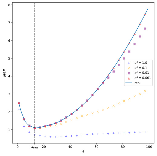
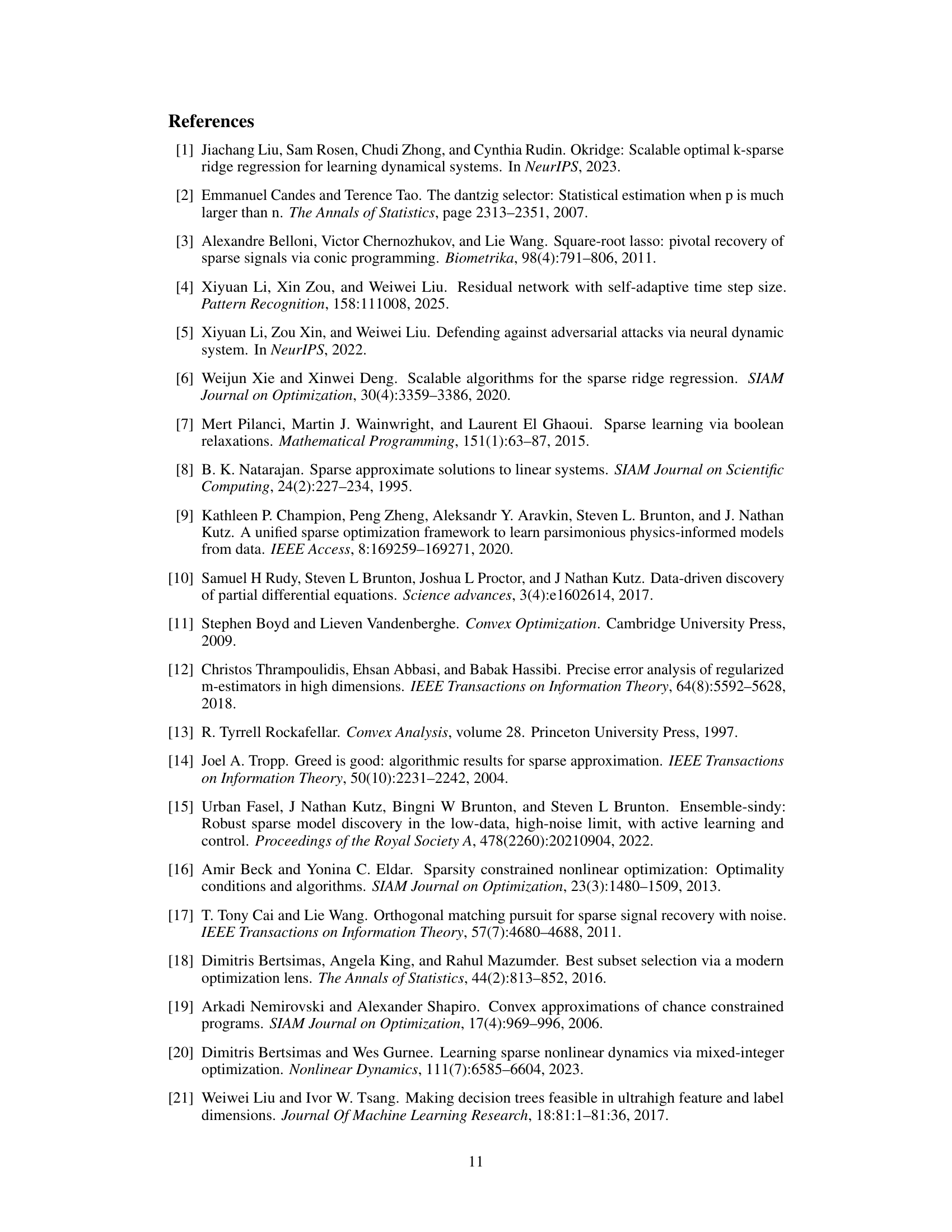
This figure shows how the Normalized Squared Error (NSE) of the OKRidge algorithm changes with respect to the regularization parameter λ for different noise levels (σ). As the noise level decreases (σ² approaches 0), the experimental NSE values (various colored markers) converge towards the theoretical curve (blue line), which represents the function ∆(λ). This convergence demonstrates that the theoretical analysis accurately predicts the algorithm’s behavior in low-noise settings. The optimal regularization parameter, denoted as λbest, is also indicated.

This figure illustrates the impact of the regularization parameter (λ) and the noise level (σ) on the normalized squared error (NSE) of the OKRidge algorithm. Multiple lines show the NSE for different values of λ as the inverse of the noise standard deviation (1/σ) increases. The bottom red line represents the NSE when λ is set to its optimal value (λbest). The figure demonstrates how NSE changes with increasing data quality (decreasing σ) for various choices of the regularization parameter, showing the algorithm’s performance converges to a specific NSE value as the noise approaches zero.
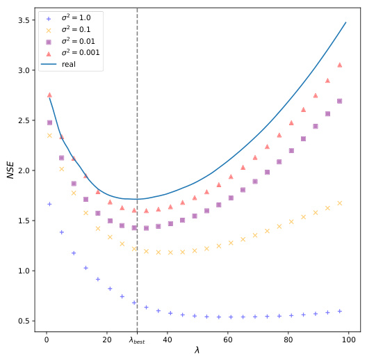
This figure shows the impact of the regularization parameter (λ) and the noise level (σ) on the normalized squared error (NSE) of the OKRidge algorithm. The x-axis represents the regularization parameter λ, and the y-axis represents the NSE. Multiple lines are plotted, each corresponding to a different noise level (σ²). As the noise level decreases (σ² approaches 0), the experimental NSE values converge to the theoretical curve (blue line) representing ∆(λ). The point λbest marks the optimal regularization parameter that minimizes NSE for a given noise level. The figure demonstrates that the NSE converges to a function of λ as noise approaches zero, aligning with the theoretical findings of the paper.
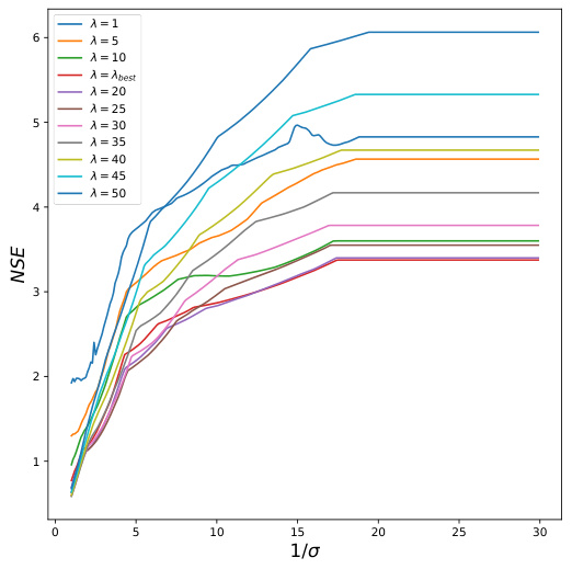
This figure shows the relationship between the Normalized Squared Error (NSE) and the inverse of the noise standard deviation (1/σ) for different values of the regularization parameter λ in the OKRidge algorithm. Each colored line represents a different value of λ, illustrating how the algorithm’s accuracy changes with varying noise levels and regularization strengths. The red line at the bottom shows the NSE when the optimal λ (λbest) is used.

This figure shows the impact of the regularization parameter (λ) and noise level (σ) on the Normalized Squared Error (NSE) of the OKRidge algorithm. Different colored lines represent different noise levels (σ² = 1.0, 0.1, 0.01, 0.001). As the noise decreases (σ² approaches 0), the experimental NSE curves converge towards the theoretical curve (in blue). The optimal λ (λbest) is indicated, highlighting the point of minimum NSE for a given noise level. The figure demonstrates the relationship between noise, regularization strength, and estimation error, supporting the theoretical findings of the paper.
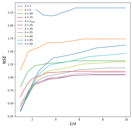
This figure shows the relationship between the Normalized Squared Error (NSE) and the inverse of the noise standard deviation (1/σ) for different values of the regularization parameter λ in the OKRidge algorithm. Each curve represents a different λ value, demonstrating how the estimation error changes as the noise level decreases. The red curve at the bottom shows the NSE when λ is set to its optimal value (λbest), highlighting the algorithm’s performance under ideal conditions.

This figure shows the relationship between the Normalized Squared Error (NSE) and the regularization parameter (λ) for different noise levels (σ). The x-axis represents λ, and the y-axis represents NSE. Multiple lines are shown, each representing a different noise level. As the noise decreases (σ approaches 0), the NSE curves converge toward a theoretical curve (blue line), indicating that the optimal λ (λbest) leads to a predictable NSE value.

This figure shows the relationship between the Normalized Squared Error (NSE) and the inverse of the noise standard deviation (1/σ) for different values of the regularization parameter λ in the OKRidge algorithm. Each curve represents a different λ value, illustrating how the NSE changes as the noise level decreases. The red curve at the bottom represents the optimal λ (λbest) and shows the best performance achievable by tuning the hyperparameter. The graph demonstrates the convergence of NSE to a fixed value as the noise level decreases for a fixed λ, a key finding in the paper.

This figure shows the change in Normalized Squared Error (NSE) as the regularization parameter (λ) varies for different noise levels (σ). The x-axis represents λ, and the y-axis represents NSE. Multiple curves are plotted, each corresponding to a different value of σ². A curve representing the theoretical limit (∆(λ)) is included for comparison. The point where λ is optimal (λbest) is also marked. The figure illustrates the impact of noise level and regularization parameter on the accuracy of the OKRidge method.

This figure shows how the Normalized Squared Error (NSE) of the OKRidge algorithm changes with respect to 1/σ (inverse of the noise standard deviation) for different values of the regularization parameter λ. Each colored line represents a different λ value. The bottom red line indicates the NSE when λ is set to its optimal value (λbest). The plot illustrates how the error behaves as noise decreases (1/σ increases) under various regularization strengths. The convergence of NSE to different values for various λ as the noise tends to zero (1/σ becomes large) is a key observation in the paper.
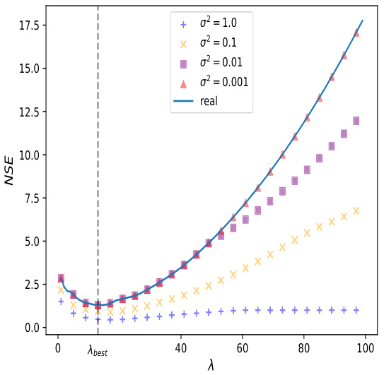
This figure shows the impact of the regularization parameter (λ) and noise level (σ) on the Normalized Squared Error (NSE) of the OKRidge algorithm. The x-axis represents the regularization parameter λ, and the y-axis represents the NSE. Multiple lines show the NSE for different values of σ². As σ² decreases, the NSE curves approach the theoretical curve (blue). This demonstrates that the NSE converges to a value determined by λ as the noise decreases, supporting the theoretical findings of the paper.

This figure shows how the Normalized Squared Error (NSE) changes with respect to 1/σ (inverse of the noise standard deviation) for different values of the regularization parameter λ in the OKRidge algorithm. Each colored line represents a different value of λ. The bottom red curve represents the best performing regularization parameter. The figure demonstrates how the NSE behaves as noise levels decrease for various regularization strengths.

This figure displays the relationship between the Normalized Squared Error (NSE) and the regularization parameter (λ) for varying noise levels (σ). Each colored line represents a different noise level (σ² = 1.0, 0.1, 0.01, 0.001), showing how NSE changes as λ increases. The blue line represents the theoretical NSE (∆(λ)). The figure demonstrates that as the noise level decreases (σ² approaches 0), the experimental NSE converges to the theoretical NSE, validating a key finding of the paper. λbest indicates the optimal value for λ which minimizes the NSE.
Full paper#

