↗ OpenReview ↗ NeurIPS Homepage ↗ Chat
TL;DR#
Extreme multi-label classification (XMC) faces challenges with massive label spaces, requiring substantial memory and computational resources. Existing methods, including dynamic sparse training (DST), often struggle with training convergence and generalization performance, especially at high sparsity levels. This is exacerbated by the highly skewed label distributions often found in real-world XMC datasets.
The researchers introduce SPARTEX, a novel approach that integrates DST with semi-structured sparsity and an auxiliary loss function. Semi-structured sparsity improves computational efficiency, while the auxiliary loss stabilizes gradient flow during the initial training phase, mitigating the challenges of poor gradient propagation. The results demonstrate significant memory savings compared to dense models, while maintaining competitive performance, even on datasets with millions of labels. SPARTEX enables end-to-end training with large label spaces on commodity hardware.
Key Takeaways#
Why does it matter?#
This paper is crucial for researchers in extreme multi-label classification (XMC) and dynamic sparse training (DST). It demonstrates the practical application of DST to XMC, a challenging domain with millions of labels, offering memory-efficient training solutions and addressing limitations of existing methods. The findings open new avenues for research in training large-scale models on commodity hardware, potentially impacting various applications dealing with high-dimensional label spaces.
Visual Insights#

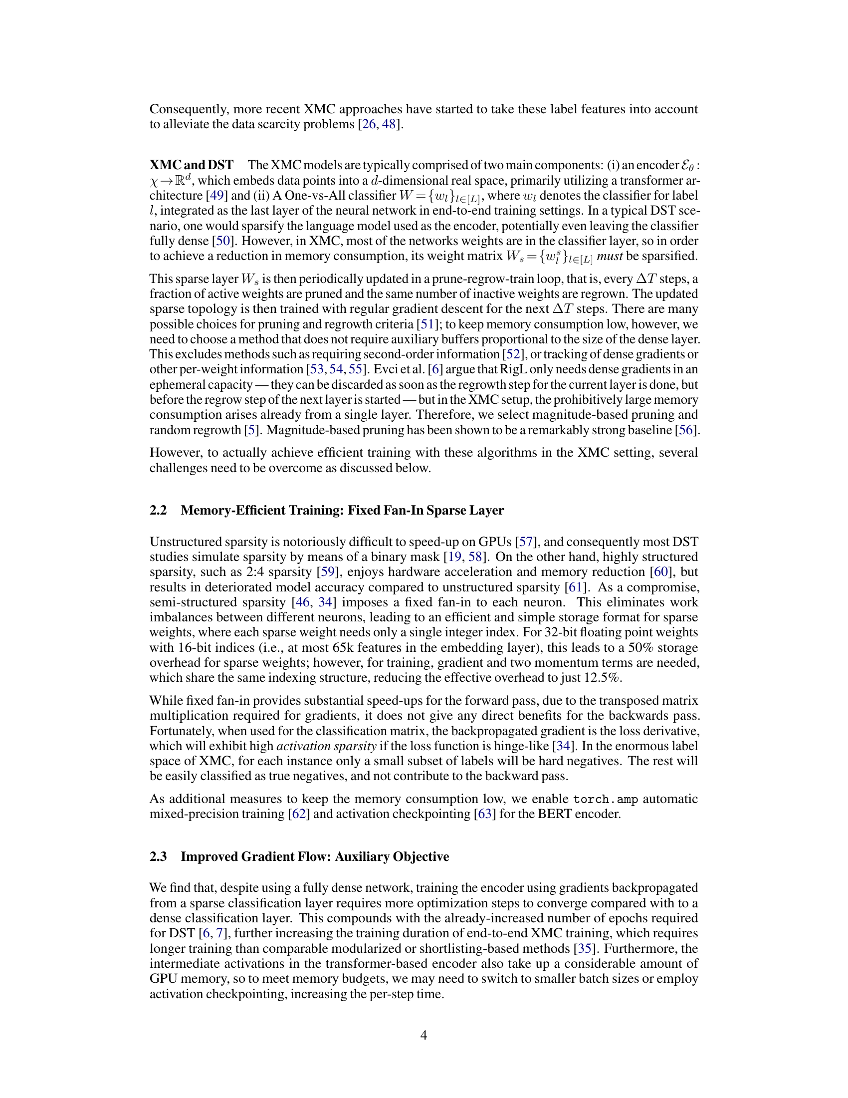
This figure shows the model architectures used in the paper and their performance compared to other methods. The left panel illustrates three variations of the model, differing in the presence of an intermediate layer and an auxiliary loss function and the size of the output space. The right panel shows a comparison of precision@1 scores on the Amazon670K dataset across varying sparsity levels, for the three model variations and two baseline approaches.

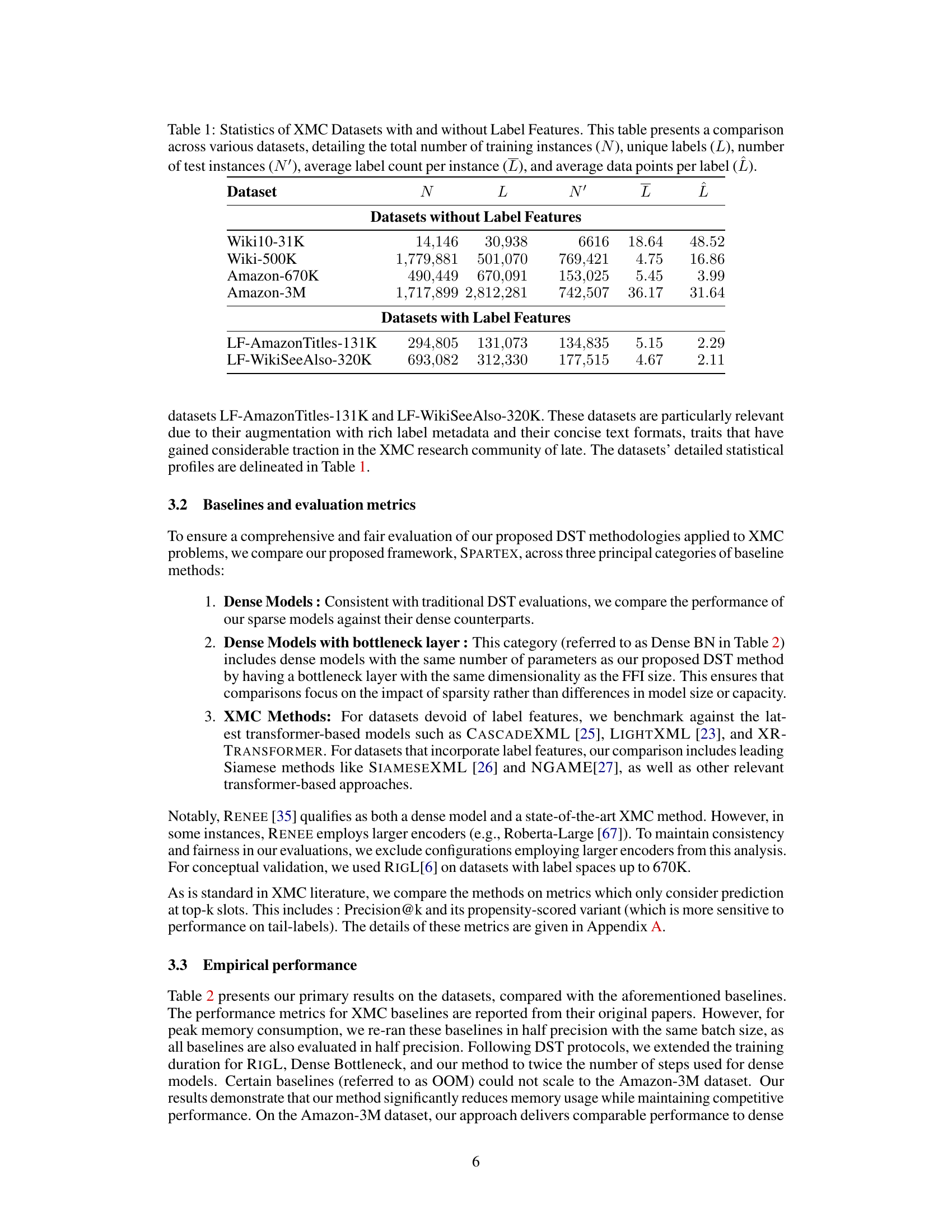
This table provides a statistical overview of several extreme multi-label classification (XMC) datasets used in the paper. It shows the number of training and testing instances, the total number of labels, the average number of labels per instance, and the average number of instances per label. The datasets are categorized into those with and without label features, offering a comparative analysis of their characteristics.
In-depth insights#
Dynamic Sparse Training#
Dynamic Sparse Training (DST) offers a compelling approach to neural network optimization by maintaining sparsity throughout the entire training process. Unlike post-training pruning, DST’s inherent sparsity leads to more memory-efficient training, though current implementations often struggle to fully realize this benefit due to the computational overhead of sparse matrix multiplication on GPUs. This paper explores DST in the challenging context of extreme multi-label classification (XMC) with large output spaces, where memory efficiency is paramount. The core challenge lies in balancing the need for sparsity with the maintenance of effective gradient flow for both the encoder and classifier. This is addressed by employing architectural modifications such as intermediate layers and auxiliary training objectives, helping to recover generalization performance while enabling end-to-end training with millions of labels on commodity hardware. The successful application of DST in this setting demonstrates its potential for addressing memory limitations in large-scale machine learning tasks.
XMC Model Efficiency#
Extreme multi-label classification (XMC) models often struggle with efficiency due to the sheer volume of labels. Memory consumption is a major bottleneck, especially during training, with classification layers demanding significant resources. This paper addresses this by exploring dynamic sparse training (DST), which maintains sparsity throughout training to reduce memory footprint. Key challenges addressed include the poor gradient flow inherent in sparse architectures and the highly skewed label distributions typical in XMC. To overcome these, the authors introduce an intermediate layer and an auxiliary training objective. The use of semi-structured sparsity with fixed fan-in also significantly boosts training efficiency on GPUs, enabling end-to-end training on commodity hardware. The results demonstrate significant memory savings compared to traditional dense models, showcasing substantial advancements in XMC model efficiency and the practical applicability of DST.
Gradient Flow Boost#
A hypothetical section titled ‘Gradient Flow Boost’ in a research paper would likely address the challenges of optimizing gradient flow, especially in complex neural network architectures. This is crucial because effective gradient flow is essential for successful training; poor gradient flow can lead to slow convergence or even training failure. The section might explore techniques to enhance gradient flow, such as introducing skip connections or residual blocks to bypass potential bottlenecks in the network. Regularization methods, like weight decay or dropout, could also be discussed as they help to prevent overfitting and improve the stability of gradient flow. Furthermore, optimizing the network architecture itself— potentially through automated search techniques or carefully chosen layer sizes and activation functions— could be presented as a means to improve gradient propagation. The impact of various training hyperparameters, such as learning rate and batch size, on gradient flow would also be analyzed. Finally, the section could feature empirical evaluations demonstrating the effectiveness of proposed gradient flow boosting techniques, comparing them against baseline methods and showcasing improvements in metrics such as training speed and model accuracy.
Auxiliary Loss Role#
The auxiliary loss in this paper is a crucial addition for stabilizing the training process of a dynamically sparse network in the context of extreme multi-label classification. Early training phases are notoriously unstable due to the noisy gradients present when working with high-dimensional, sparse layers. The auxiliary loss helps address this by providing a more stable and informative gradient signal during these initial stages. It does so by employing a coarser-grained objective, which helps the encoder learn effective representations. This auxiliary objective is eventually turned off once the network has learned a sufficiently good representation, to avoid misalignment with the primary task. The choice of a meta-classifier based loss is particularly clever, leveraging the existing clustering structure commonly used in XMC to provide a smooth transition to the main objective. It highlights how smart design choices in the loss function can compensate for the inherent difficulties of training sparse models in a challenging domain.
Future Research#
Future research directions stemming from this work on dynamic sparse training for extreme multi-label classification could focus on several key areas. Improving the efficiency of sparse training algorithms remains paramount; exploring novel pruning and regrowth strategies beyond SET could yield significant benefits. Further investigation into the interplay between sparsity levels and the label distribution’s long-tailed nature is warranted. Developing more sophisticated methods for managing gradient flow through sparse layers, potentially leveraging advanced optimization techniques or architectural innovations, deserves attention. The impact of different sparsity patterns and architectures beyond fixed fan-in semi-structured sparsity should be investigated. Finally, extending the approach to even larger-scale problems and diverse data modalities, while maintaining efficiency and accuracy, presents an exciting challenge. Investigating the use of more powerful encoder architectures may be beneficial in this regard.
More visual insights#
More on figures
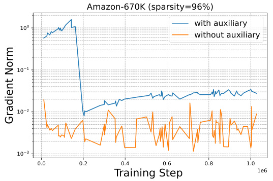
This figure compares the gradient flow of the encoder during training with and without the auxiliary objective. The plot shows that the introduction of an auxiliary objective results in a significantly larger gradient signal during the initial training phase, which speeds up learning. However, because the task associated with the meta-classifiers differs from the final task, while both share the same encoder, maintaining it throughout the entire training process can deteriorate the encoder’s representation quality. Therefore, the auxiliary objective’s influence is gradually reduced as training progresses.
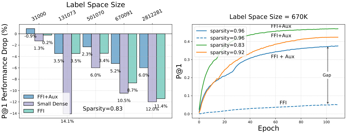
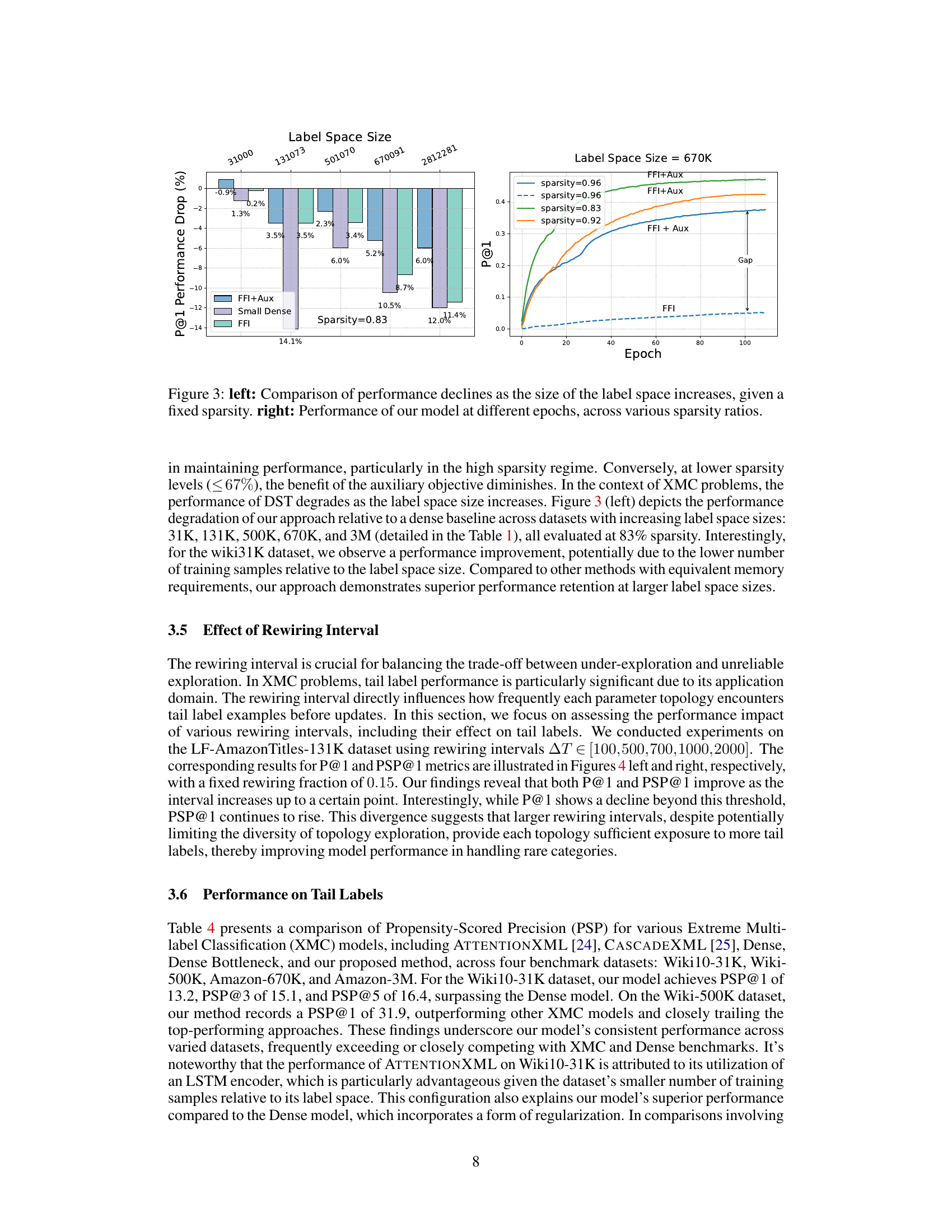
The figure shows a comparison of performance degradation in DST as the size of the label space increases. The left panel shows the performance drop at a fixed sparsity level (83%) across different label space sizes (31K, 131K, 500K, 670K, 3M). The right panel shows the performance of the model at different epochs and sparsity levels (83%, 92%, and 96%) for the Amazon-670K dataset. It highlights the impact of label space size and sparsity on model performance.
This figure presents a comparison of different model configurations for dynamic sparse training (DST) and their performance across various sparsity levels. The left panel shows the model architectures with a semi-structured sparse layer (‘S’), an intermediate layer (‘W’), and an auxiliary head (‘Aux’). The right panel shows a graph comparing the precision@1 of the proposed method and other baselines as sparsity increases on the Amazon670K dataset.
This figure shows the model architecture used in the paper (left panel) and a comparison of its performance against other methods on the Amazon670K dataset (right panel). The architecture uses a combination of semi-structured sparse layer, intermediate layer, and an auxiliary head, which helps improve performance at high sparsity levels and large output spaces. The comparison shows that the proposed model achieves competitive precision@1 results.

This figure shows the model architectures used in the paper for various sparsity levels and label space sizes. The left panel illustrates the different components of the model, including the semi-structured sparse layer (S), intermediate layer (W), and auxiliary head (Aux). The right panel compares the precision@1 of the proposed model with other methods, demonstrating its ability to maintain performance at higher sparsity levels and larger label spaces.

This figure shows the model architecture and performance comparison. The left panel illustrates three model variations: a baseline with only a semi-structured sparse layer (S), a model adding an intermediate layer (W), and a model using an auxiliary classifier (Aux). The right panel compares the precision@1 of the three variations against a dense model and a static sparsity model across a range of sparsity levels, demonstrating the effectiveness of the proposed architecture in maintaining performance, particularly at high sparsity levels and large label spaces.
More on tables
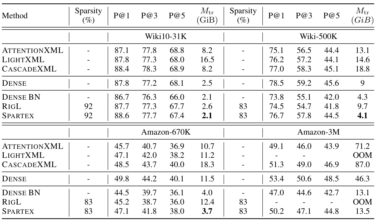
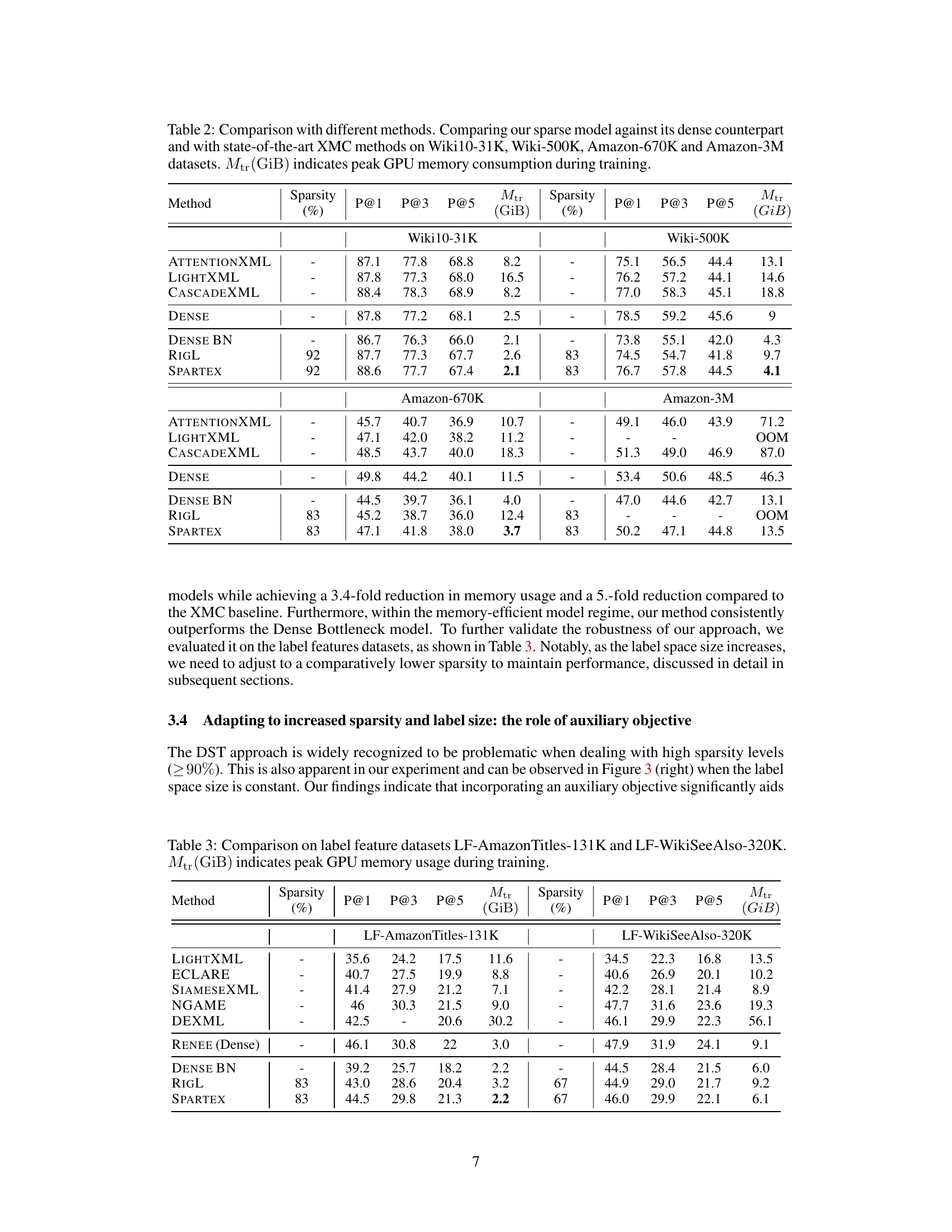
This table compares the performance of the proposed Dynamic Sparse Training (DST) method against several baseline methods across four different extreme multi-label classification (XMC) datasets. The baselines include dense models, dense models with a bottleneck layer, and state-of-the-art XMC methods. The table shows precision at 1, 3, and 5, along with the peak GPU memory consumption during training for each method and dataset. The sparsity level of the DST method is also indicated.
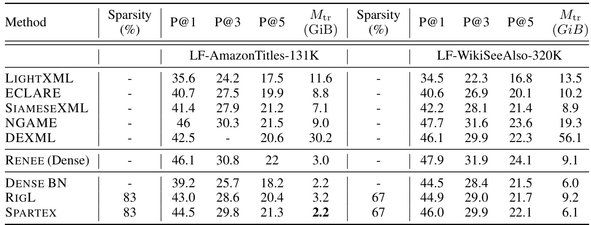
This table compares the performance of the proposed Dynamic Sparse Training (DST) method against several baselines on four extreme multi-label classification (XMC) datasets. The baselines include dense models, dense models with a bottleneck layer, and other state-of-the-art XMC methods. The table shows precision at 1, 3, and 5, as well as the peak GPU memory consumption during training for each method. The sparsity level is also indicated for the sparse methods.
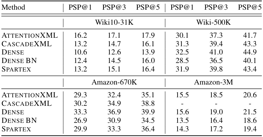
This table compares the performance of the proposed SPARTEX model against various baselines on four extreme multi-label classification (XMC) datasets. Baselines include dense models, dense models with a bottleneck layer, and state-of-the-art XMC methods. The table shows precision at 1, 3, and 5, and peak GPU memory consumption (Mtr) during training, for various sparsity levels. It highlights the memory efficiency of the proposed method while maintaining competitive performance.
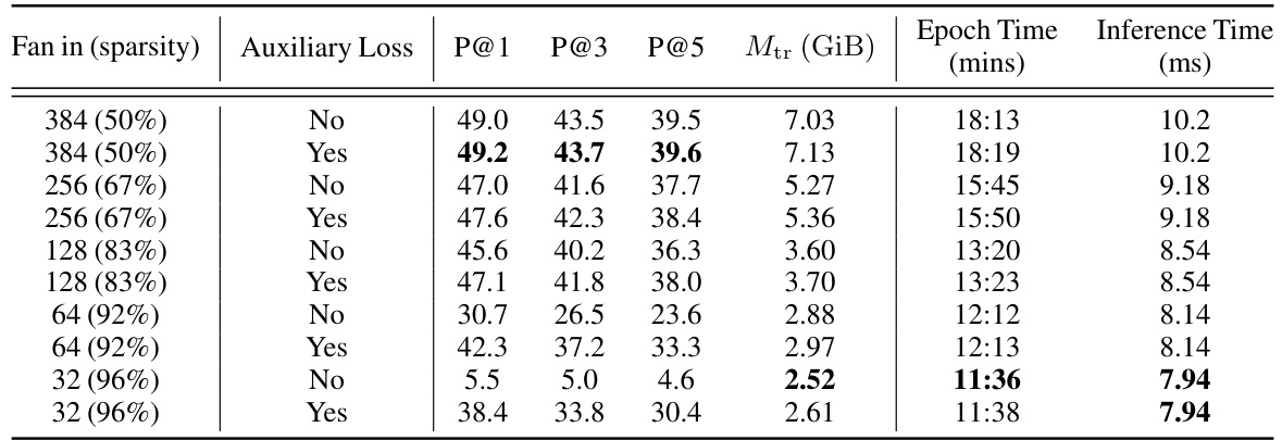
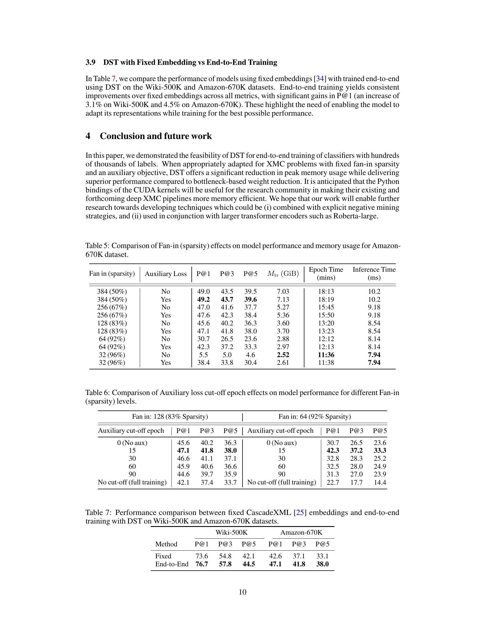
This table shows the impact of different sparsity levels (controlled by the fan-in parameter) and the use of an auxiliary loss on the performance (P@1, P@3, P@5) and memory usage (Mtr) for the Amazon-670K dataset. It also provides the training time (Epoch Time) and inference time (Inference Time) for each configuration, demonstrating the trade-off between model sparsity, performance, and resource consumption.

This table shows the impact of varying the cut-off epoch for the auxiliary loss on the model’s final performance. Two different sparsity levels (83% and 92%) are considered. The results are presented in terms of Precision@1 (P@1), Precision@3 (P@3), and Precision@5 (P@5). It shows that there is an optimal cut-off point for the auxiliary loss, beyond which, performance begins to degrade.

This table compares the performance of models using fixed embeddings (CascadeXML) with end-to-end training using Dynamic Sparse Training (DST) on two datasets: Wiki-500K and Amazon-670K. It shows that end-to-end training with DST leads to consistent improvements over using fixed embeddings across all metrics (Precision@1, Precision@3, Precision@5). The gains are more significant for Precision@1.

This table lists the hyperparameters used in the experiments for different datasets. It specifies the encoder architecture (BERT Base or DistilBERT), batch size, dropout rate, number of training epochs, learning rates for the encoder and classifier, warmup steps, and sequence length.
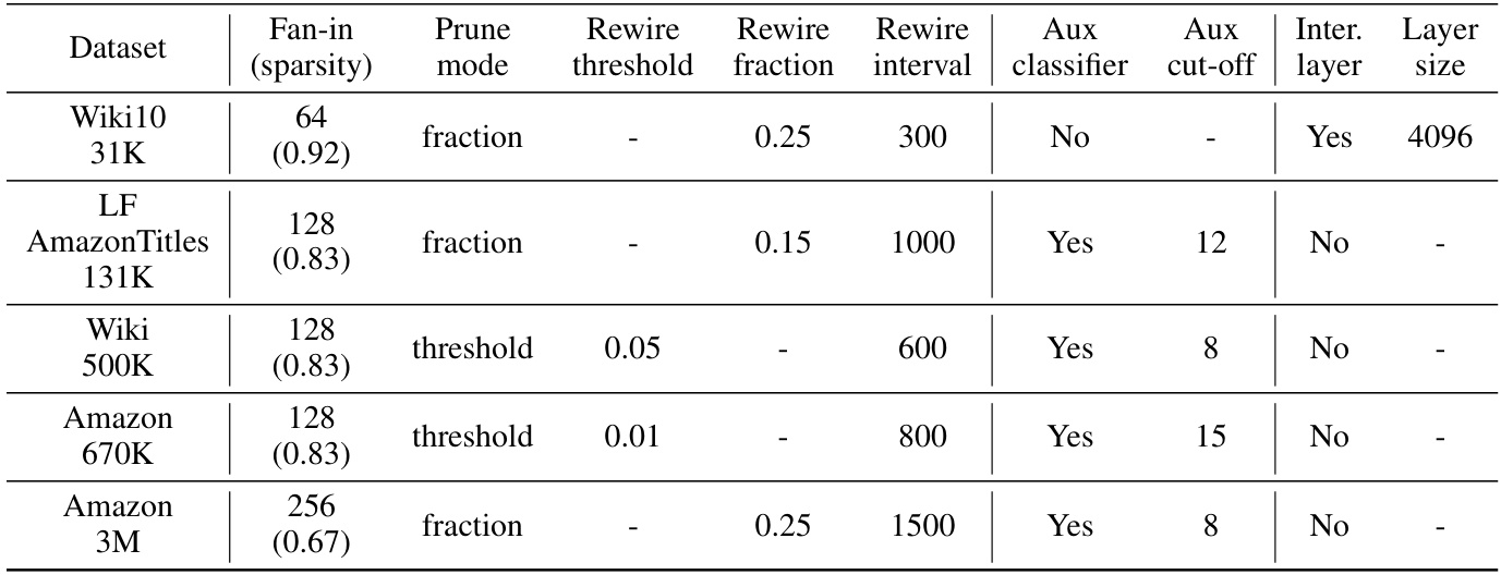
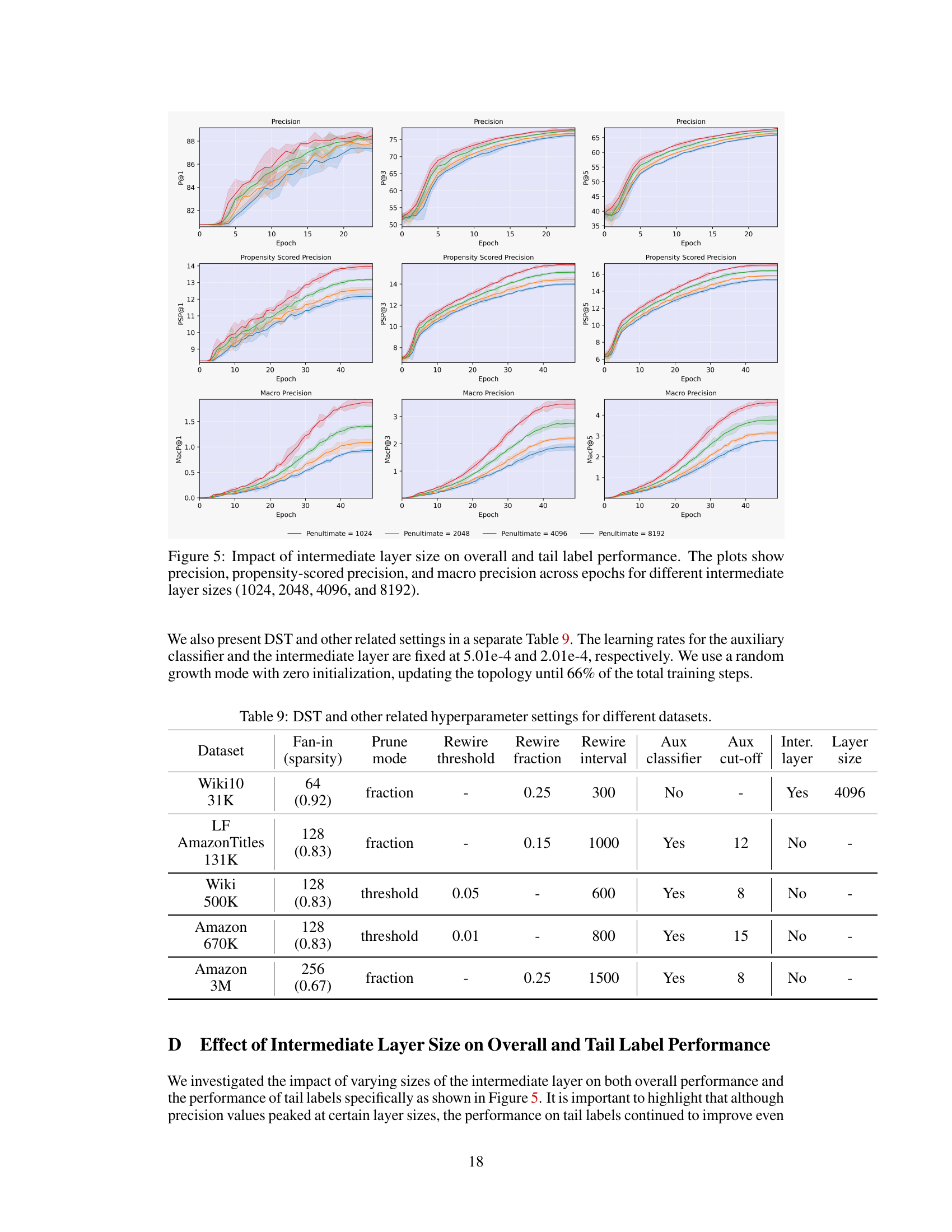
This table details the hyperparameters used in the Dynamic Sparse Training (DST) experiments across different datasets. It shows the fan-in (sparsity level), pruning mode (fraction or threshold), rewiring threshold and fraction, rewiring interval, use of an auxiliary classifier, auxiliary loss cut-off epoch, and whether an intermediate layer was used and its size. These parameters were adjusted for each dataset to optimize training efficiency and performance.
Full paper#
