↗ OpenReview ↗ NeurIPS Homepage ↗ Chat
TL;DR#
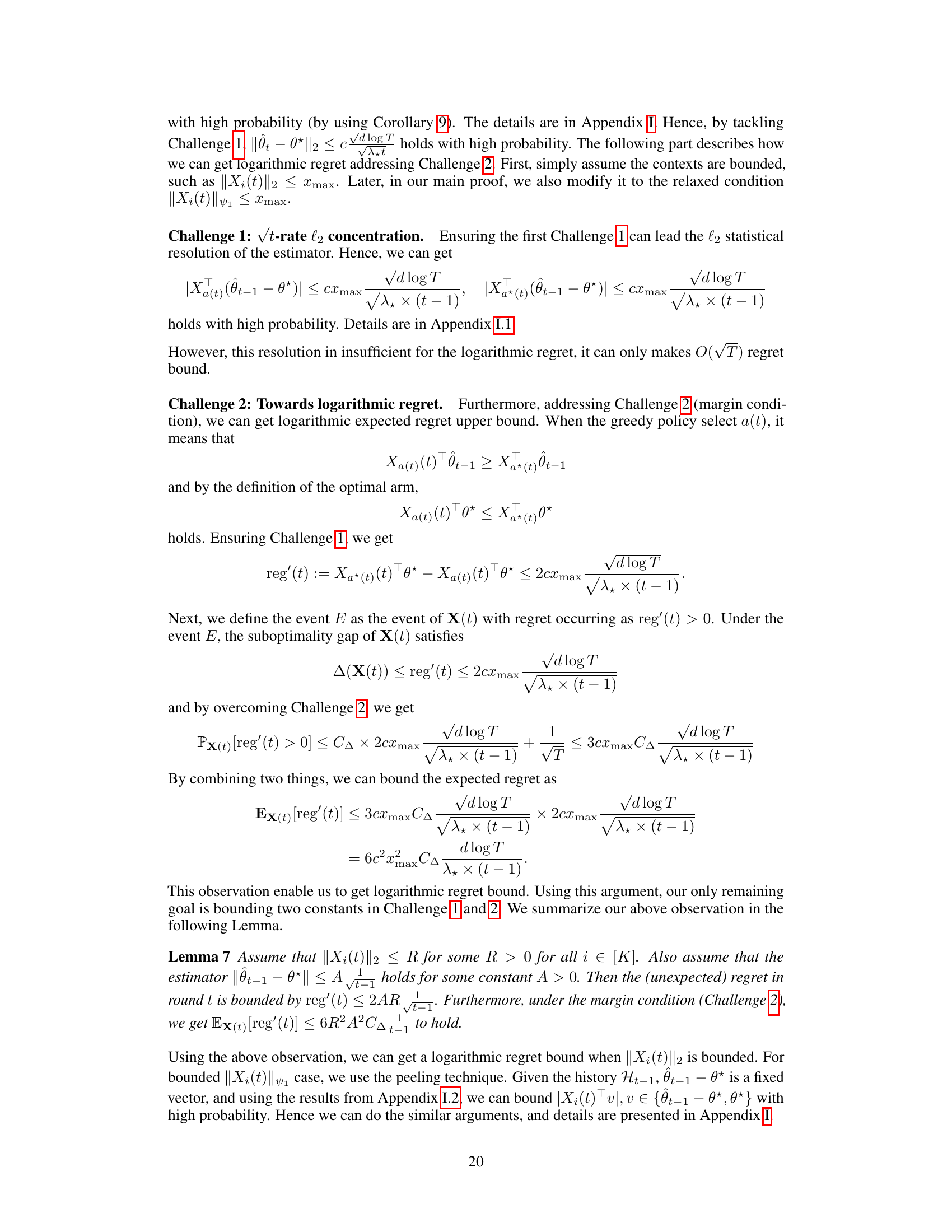
Linear contextual bandits require balancing exploration and exploitation to maximize cumulative rewards. Existing efficient exploration-free greedy algorithms were limited to Gaussian and uniform distributions, thus limiting real-world application. This restriction hinders progress in situations where exploration is costly or impractical.
This paper introduces a new condition, Local Anti-Concentration (LAC), enabling efficient greedy algorithms for a wider range of distributions. The LAC condition guarantees a poly-logarithmic regret bound (O(poly log T)), meaning the algorithm performs efficiently even without exploration. This is a significant step forward, expanding the applicability of simple, computationally efficient greedy strategies to many more real-world scenarios.
Key Takeaways#
Why does it matter?#
This paper is crucial because it significantly expands the range of distributions for which exploration-free greedy algorithms are provably efficient. This addresses a major limitation in the field, enabling broader application of these computationally cheaper methods and opening avenues for future work in similar settings.
Visual Insights#

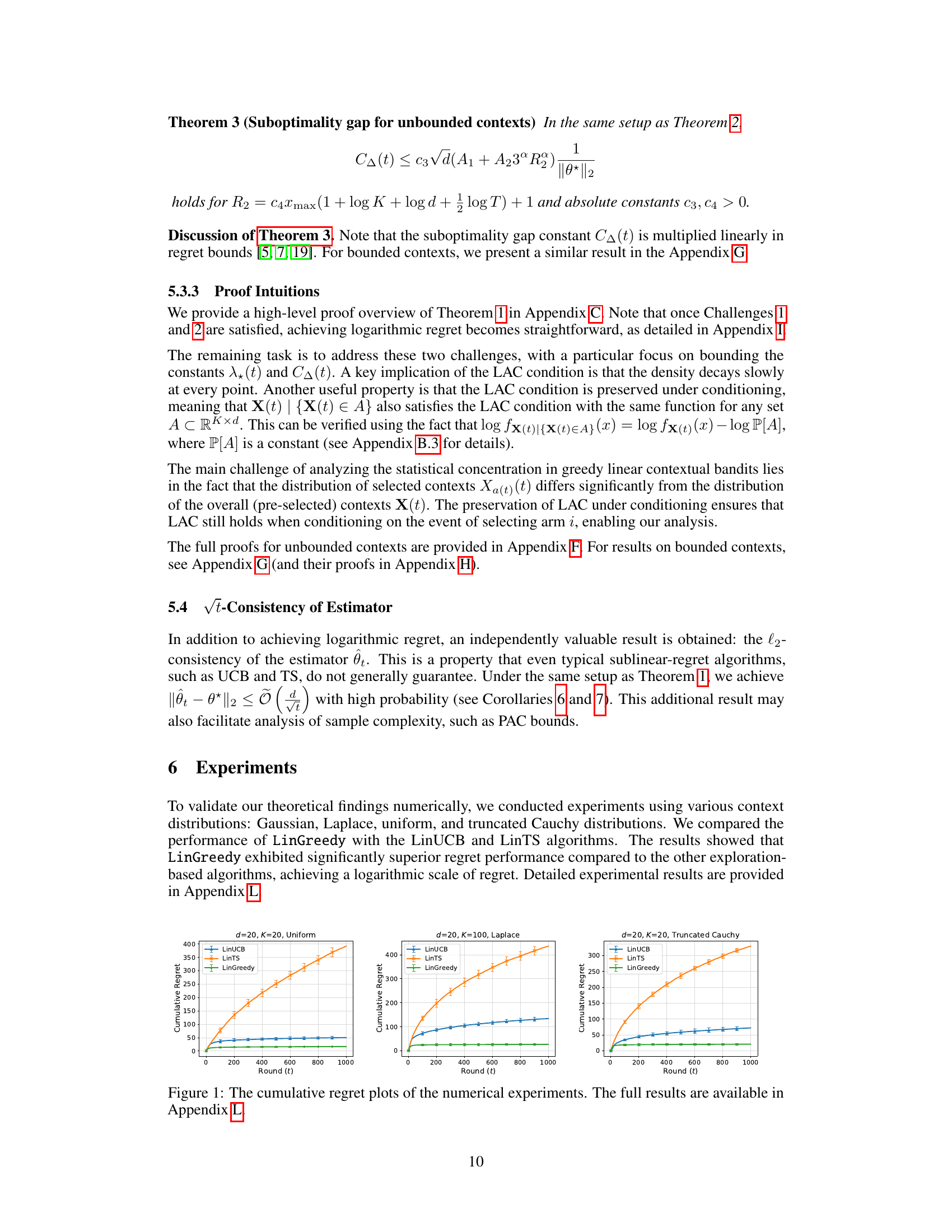
The figure shows the cumulative regret plots for three different experimental settings, each with a different context distribution (Uniform, Laplace, and Truncated Cauchy). Each plot compares the performance of three algorithms: LinUCB, LinTS, and LinGreedy. The results in the figure are a subset of the more extensive numerical experiments reported in Appendix L of the paper.
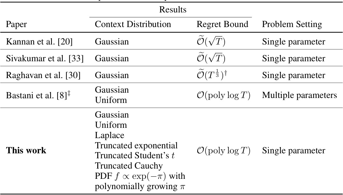
This table compares several studies on greedy linear contextual bandit algorithms. It lists the context distribution used in each study (mostly Gaussian), the achieved regret bound (ranging from O(√T) to O(poly log T)), and the problem setting (single parameter or multiple parameters). The table highlights the expansion of applicable distributions from mostly Gaussian and uniform in previous works to a significantly wider class including Gaussian, exponential, uniform, Cauchy, Student’s t, and their truncated variants in the current work. The poly-logarithmic regret bound represents a significant improvement in efficiency.
In-depth insights#
LAC Condition#
The Local Anti-Concentration (LAC) condition, a novel contribution of this research paper, is a crucial criterion for establishing the efficiency of exploration-free greedy algorithms in linear contextual bandit settings. It relaxes the stringent requirements of existing methods, which primarily focused on Gaussian or uniform data distributions, by broadening the scope to include a wider array of distributions: Gaussian, exponential, uniform, Cauchy, Student’s t, and their truncated counterparts. This expansion significantly increases the applicability and practicality of greedy approaches. The LAC condition is cleverly defined using the log density function and its properties, ensuring it is both mathematically sound and computationally tractable. Crucially, the LAC condition facilitates a sharper regret guarantee, achieving poly-logarithmic regret, a substantial improvement over previous findings that were mostly limited to O(√T) regret. Furthermore, the theoretical analysis elegantly demonstrates that the LAC condition implicitly implies essential properties, such as the growth of the minimum eigenvalue of the Gram matrix and probabilistic boundedness of the suboptimality gap, which were previously assumed as independent conditions.
LinGreedy Analysis#
LinGreedy analysis delves into the theoretical underpinnings of a novel exploration-free algorithm for linear contextual bandits. A core aspect is the introduction of the Local Anti-Concentration (LAC) condition, a novel criterion for distribution of contexts that enables the algorithm to achieve strong performance guarantees, expanding beyond the limited Gaussian and uniform distributions previously considered. The analysis rigorously establishes a polylogarithmic regret bound under LAC, showcasing its efficiency. This bound is tighter than prior results for greedy approaches, highlighting a significant advancement. The analysis overcomes key challenges in proving efficiency for greedy linear bandits, including ensuring sufficient diversity in the adapted Gram matrix and bounding the suboptimality gap, without assuming these properties a priori. Theorems are provided to substantiate the key claims regarding regret bounds, the diversity constant, and the suboptimality gap, highlighting the technical depth of the analysis and its reliance on carefully developed techniques, including the use of concentration inequalities and martingale arguments. The work presents significant theoretical contributions to the field of contextual bandits.
Regret Guarantees#
Regret guarantees in the context of online learning algorithms, particularly in bandit settings, are crucial for evaluating performance. They quantify the difference between the cumulative reward obtained by an algorithm and the optimal reward achievable with perfect knowledge. The paper likely focuses on analyzing the cumulative regret of a greedy algorithm, which is exploration-free, a significant challenge because such algorithms, by design, do not explicitly explore suboptimal actions to learn about their true values. The core of the regret analysis likely involves demonstrating that, under specific distributional assumptions (such as the Local Anti-Concentration condition introduced in this paper), the algorithm’s regret grows sublinearly, ideally achieving a poly-logarithmic bound with the number of time steps. This implies that while the algorithm doesn’t explore, the structure of the problem (context diversity and distributional properties) helps ensure it performs well, making the exploration step unnecessary. The significance of this lies in practical application, as exploration is often costly, time-consuming, or even infeasible. A solid regret guarantee indicates that the greedy algorithm is indeed efficient despite its lack of exploration, extending the applicability of simpler, exploration-free methods beyond commonly considered settings.
Empirical Results#
An effective ‘Empirical Results’ section in a research paper would go beyond simply presenting numbers; it would offer a thorough analysis interpreting the findings within the study’s context. It should start with a clear, concise overview of the key results, highlighting the most significant findings and their implications. Next, it should systematically present the detailed results, using appropriate visualizations (tables, graphs, etc.) to improve clarity and facilitate understanding. Crucially, the discussion should address any unexpected or counterintuitive results, explaining potential reasons and acknowledging any limitations. Statistical significance should be explicitly stated, indicating whether observed effects are likely due to chance or represent genuine phenomena. Furthermore, a robust ‘Empirical Results’ section will compare the obtained results with prior work, highlighting both similarities and differences and situating the current study within the broader literature. Finally, future research directions should be suggested based on the results and any open questions that remain.
Future Work#
The paper’s ‘Future Work’ section could explore several promising avenues. Extending the Local Anti-Concentration (LAC) condition to a broader range of distributions, including those with heavier tails or discrete support, would significantly enhance the applicability of greedy algorithms. Investigating the impact of context correlations on the LAC condition and exploring methods to handle correlated contexts efficiently is crucial. A detailed empirical comparison of greedy methods against exploration-based approaches across diverse datasets and problem settings would validate the theoretical findings and highlight the practical advantages of greedy algorithms under specific conditions. Finally, theoretically analyzing the impact of different noise models on the regret bound could provide valuable insights into the robustness of greedy methods and inform the design of more robust algorithms. This rigorous analysis would further refine our understanding of the conditions under which exploration-free greedy strategies excel.
More visual insights#
More on figures
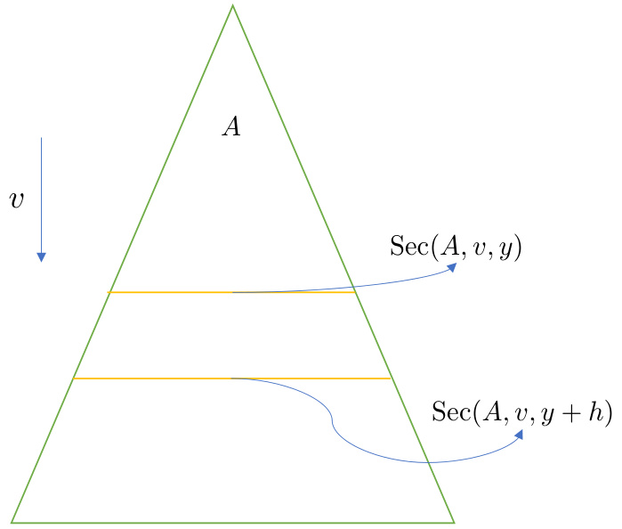
The figure illustrates the concept of expanding sections. A section is defined as the intersection of a region A and a hyperplane. In the context of expanding sections, as the value of y increases, the size of the intersection (the section) also increases. This figure uses a triangle to demonstrate this idea. The section at y + h is clearly larger than that at y, showing that the size of the section expands with y.
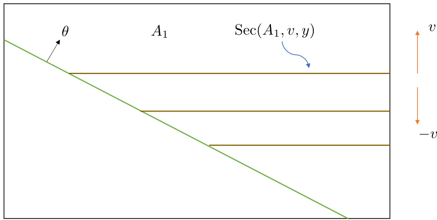
This figure illustrates the concept of expanding sections. The main part shows a set A (green region), a direction vector v (orange arrow), and several parallel hyperplanes perpendicular to v. The brown lines represent the intersections of the hyperplanes with set A, which are labeled as Sec(A, v, y). These sections are expanding as the value of y increases, which is important for Lemma 8 in the paper that establishes a one-sided decay rate.

This figure illustrates different types of sections within a ball in d-dimensional space (BR). It highlights two specific section types: SR(0, b, v, y) shown as a red line and SR(0, b) shown as a green line. The figure is used in the context of discussing how linear section maps are constructed between sections of the ball in order to analyze the one-sided decay rate of section densities for bounded contexts in a linear contextual bandit setting.
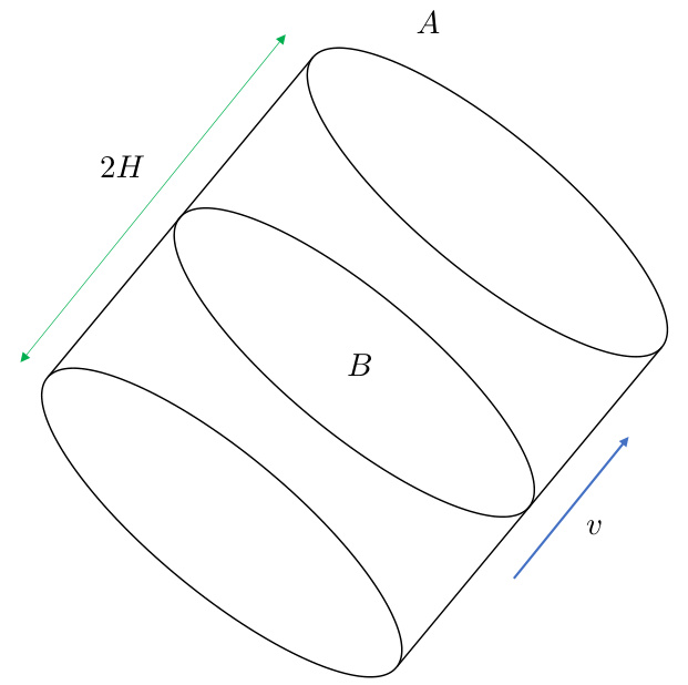
This figure illustrates a cylindrical region A in d-dimensional space. The region is defined by a base B (a subset of a hyperplane orthogonal to vector v), and a length 2H along the direction of vector v. The region A is the set of all points that can be expressed as B + tv for -H ≤ t ≤ H, where t is a scalar.
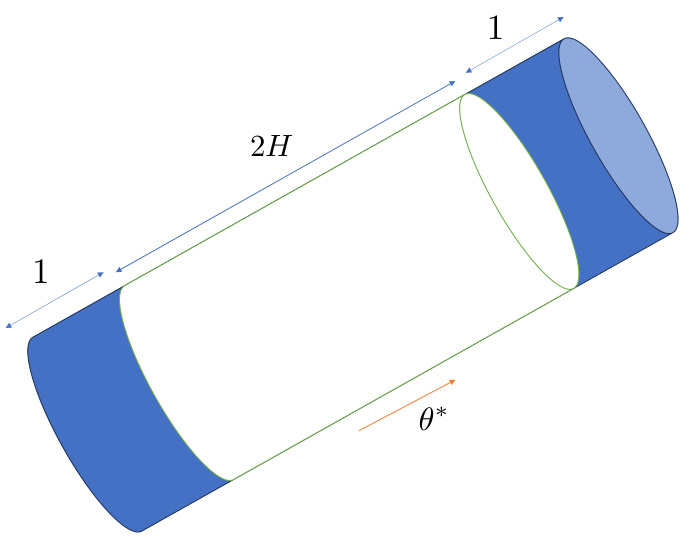
This figure illustrates the support of Zi, which is a cylindrical set with length 2H and radius R. The support has equal sections with direction θ*. This is a key geometric property used in the proof of Proposition 3, which provides a bound on the margin constant C△ in the context of the fixed-history setup.
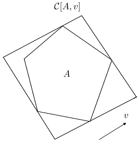
This figure illustrates the set completion operation, denoted as C[A, v]. Given a set A and a vector v, the operation expands A such that all sections parallel to the hyperplane perpendicular to v have equal size. The figure shows a polygon A and the result of applying the C[A, v] operation, resulting in a larger polygon with parallel sides in the direction of v.
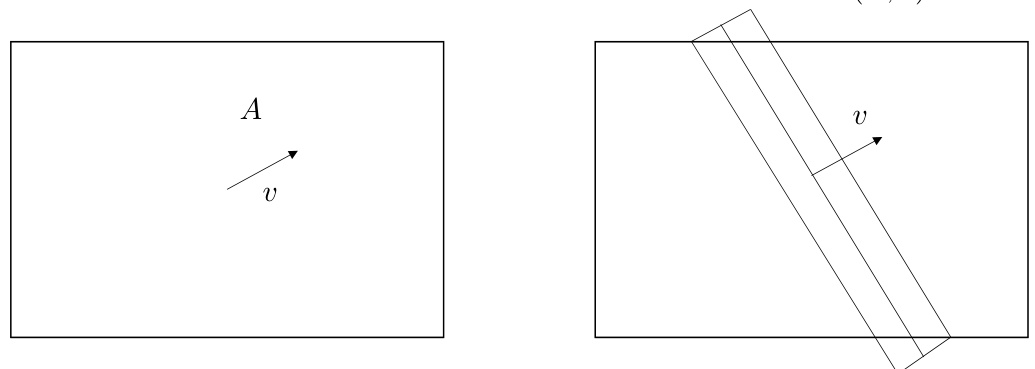
The figure shows the operation of filling an area A in a specific direction v. The process ensures that all cross-sections of the resulting shape are equal when cut by a hyperplane orthogonal to the direction v. The left panel shows the initial area A, and the right panel illustrates the operation of filling A. This process modifies the shape to make its cross-sections uniform along the direction v.
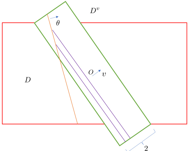
The figure illustrates the construction of the set Dº, a crucial element in the proof of Theorem 2. The red rectangle represents the initial set D, which is a hypercube. The green parallelogram, Dº, is created by extending D along the direction of vector v until equal sections are achieved within the interval [-1, 1] along v. This process ensures that the assumptions of Proposition 2 are satisfied and that the results can be applied.
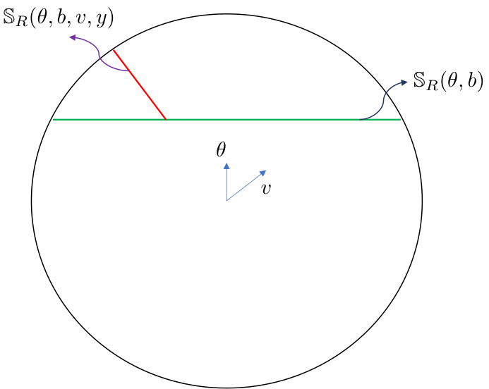
This figure illustrates different sections of a d-dimensional ball with radius R, denoted as BR. It highlights the key sections used in the paper’s analysis of the greedy algorithm for bounded contexts. The green line represents a section of the ball defined by the hyperplane {x ∈ BR | x⋅θ = b}, where θ is a vector and b is a scalar. The purple curve represents a section defined by the hyperplane {x ∈ BR | x⋅v = y}, where v is a vector and y is a scalar. Finally, the red line shows the intersection of these two sections, denoted as SR(θ, b, v, y), which represents the area used for analyzing the one-sided decay rate of section density in the analysis of the greedy algorithm for bounded contexts.

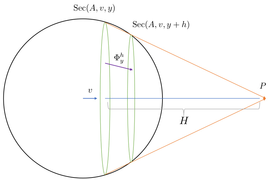
The figure illustrates the concept of a projection map, a type of affine point projection. The projection map is shown as a transformation from a set A to a point P. The projection point P determines the direction of the projection, and all points in A are projected toward P.
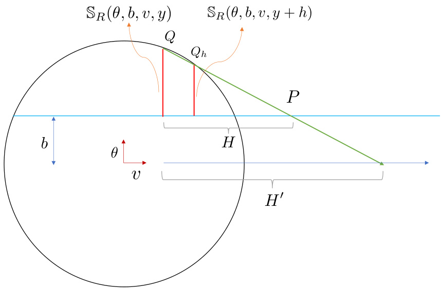
This figure illustrates different sections of a ball in a d-dimensional space. The main section is the ball itself, represented by the larger circle. Within the ball, two types of sections are highlighted. The green line, denoted as SR(0, b), represents a section created by a hyperplane (a plane) that is perpendicular to vector θ and passes through a point at a distance b from the origin along θ. The red line, denoted as SR(0, b, v, y), is a more complex section which is created by intersecting the ball with two hyperplanes; the first hyperplane is perpendicular to vector θ and passes through a point at a distance b from the origin along vector θ, while the second hyperplane is perpendicular to vector v and passes through a point at a distance y from the origin along vector v. This detailed illustration of sections is essential for the mathematical analysis of the paper, particularly in bounding the one-sided decay rate of section density for bounded contexts.

This figure illustrates different types of sections within a ball with radius R in a d-dimensional space. The sections are created by intersecting the ball with hyperplanes and considering specific constraints. The sections are used in the paper to mathematically analyze the behavior of greedy algorithms under different conditions. The red line represents SR(θ, b, v, y), a section created using a hyperplane defined by vector v and a threshold value y, constrained to also satisfy a condition involving vector θ and threshold b. The green line represents SR(θ, b), a different section based only on θ and b. Understanding these section types and their properties is crucial to analyzing the theoretical aspects of the greedy algorithms.
This figure illustrates different types of sections within a ball with radius R in d-dimensional space. It highlights the sections created by intersecting the ball with hyperplanes. The sections are defined as follows: * SR(θ, b): The intersection of the ball with the half-space defined by the hyperplane xᵀθ ≥ b, where θ is a direction vector and b is a threshold value. * SR(v, y): The intersection of the ball with the hyperplane xᵀv = y, where v is a direction vector and y is a value. * SR(θ, b, v, y): The intersection of the ball with both the hyperplane xᵀθ ≥ b and the hyperplane xᵀv = y. This is a more complex section that is a subset of the SR(θ, b) section. The figure visually demonstrates these sections, showing how the shapes change depending on the relative orientations of θ and v and the values of b and y.
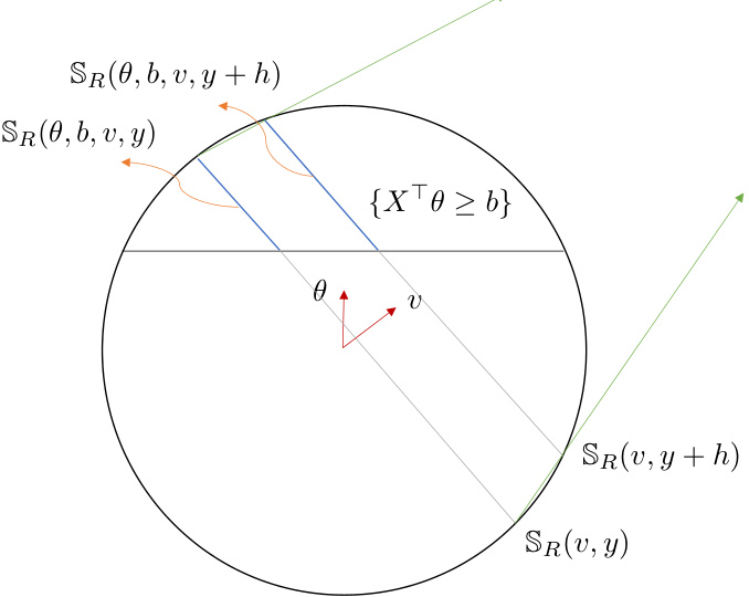
This figure illustrates different sections of a ball in a d-dimensional space. It shows how the sections are created by intersecting the ball with hyperplanes defined by vectors v and θ. Specifically, it highlights: * SR(v, y): A sliced ball – the intersection of the ball with a hyperplane perpendicular to vector v at distance y from the origin. * SR(θ, b): The intersection of the ball with a half-space defined by the hyperplane with normal vector θ and passing through a point at a distance b from the origin, such that xTθ ≥ b. * SR(θ, b, v, y): A double-sliced ball - the intersection of the ball with both the half-space (xTθ ≥ b) and the hyperplane perpendicular to v at distance y from the origin. The figure is crucial for understanding the analysis in Section H.2 and H.6, which addresses how to manage the one-sided decay rate of section densities in bounded contexts. The different sections represent different scenarios considered in analyzing the behavior of the greedy algorithm, especially when dealing with boundary cases, i.e., not just the interior of the ball but also near the edges.

This figure shows the cumulative regret of three different algorithms (LinUCB, LinTS, and LinGreedy) across different numbers of rounds (t). The results are shown for four different context distributions (Gaussian, Uniform, Laplace, and Truncated Cauchy) and three different parameter settings (d=20, K=20; d=20, K=100; d=100, K=20). The plots demonstrate that the LinGreedy algorithm, which is exploration-free, significantly outperforms the other two exploration-based algorithms in all cases. Appendix L provides further details and additional results.

The figure shows the cumulative regret for three different experimental settings. Each setting varies the distribution of contexts (Uniform, Laplace, Truncated Cauchy), using a dimension (d) of 20 and a number of arms (K) of 20 for the first set, d=20 and K=100 for the second and d=100 and K=20 for the third set. The plots compare the performance of LinGreedy against LinUCB and LinTS algorithms. LinGreedy consistently shows lower cumulative regret, indicating its effectiveness in these scenarios. More detailed results are available in Appendix L.
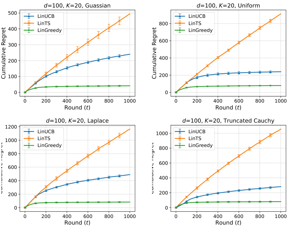
This figure shows the cumulative regret for three different experimental settings (d=20, K=20; d=20, K=100; d=20, K=20) across various context distributions (Uniform, Laplace, Truncated Cauchy). Each setting compares the performance of three algorithms: LinUCB, LinTS, and LinGreedy. The plots visualize the cumulative regret over a number of rounds, illustrating the relative performance of the different algorithms under different distributional assumptions. Details of these experiments are in Appendix L.
Full paper#

