↗ OpenReview ↗ NeurIPS Homepage ↗ Chat
TL;DR#
Estimating the impact of treatments from observational data is challenging because it’s difficult to account for randomness in treatment effects. This is important because simply knowing the average treatment effect doesn’t tell the full story. This paper focuses on quantifying this randomness (aleatoric uncertainty) which is important for understanding the probability of success or other quantiles. Current machine learning methods for causal inference mostly focus on average treatment effects and haven’t paid much attention to this variability.
This work introduces a novel method, called the AU-learner, to address this issue. The AU-learner uses a technique called partial identification to get sharp bounds on the aleatoric uncertainty. It’s also designed to be robust to errors in the data, a crucial property for real-world applications. The researchers show through experiments that their approach performs well and has several advantages compared to existing techniques. The use of conditional normalizing flows provides a practical way to implement the AU-learner.
Key Takeaways#
Why does it matter?#
This paper is crucial for researchers working with observational data to understand treatment effects. It addresses a significant gap by focusing on aleatoric uncertainty, providing novel methods for estimating the conditional distribution of treatment effect (CDTE), which is not typically addressed in causal inference. The proposed orthogonal learner offers strong theoretical guarantees and practical advantages, paving the way for improved decision-making in various fields.
Visual Insights#

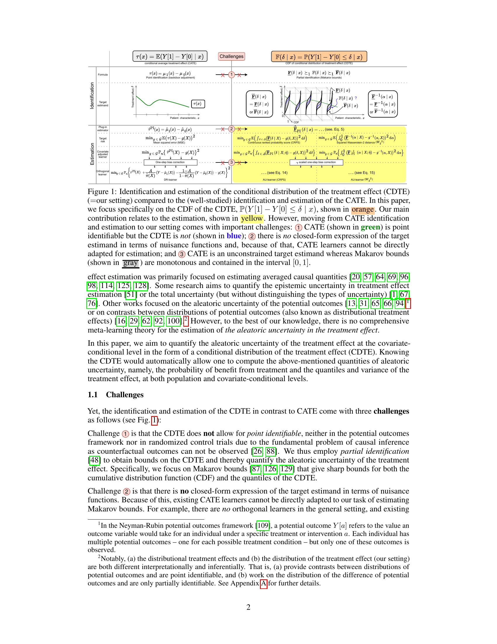
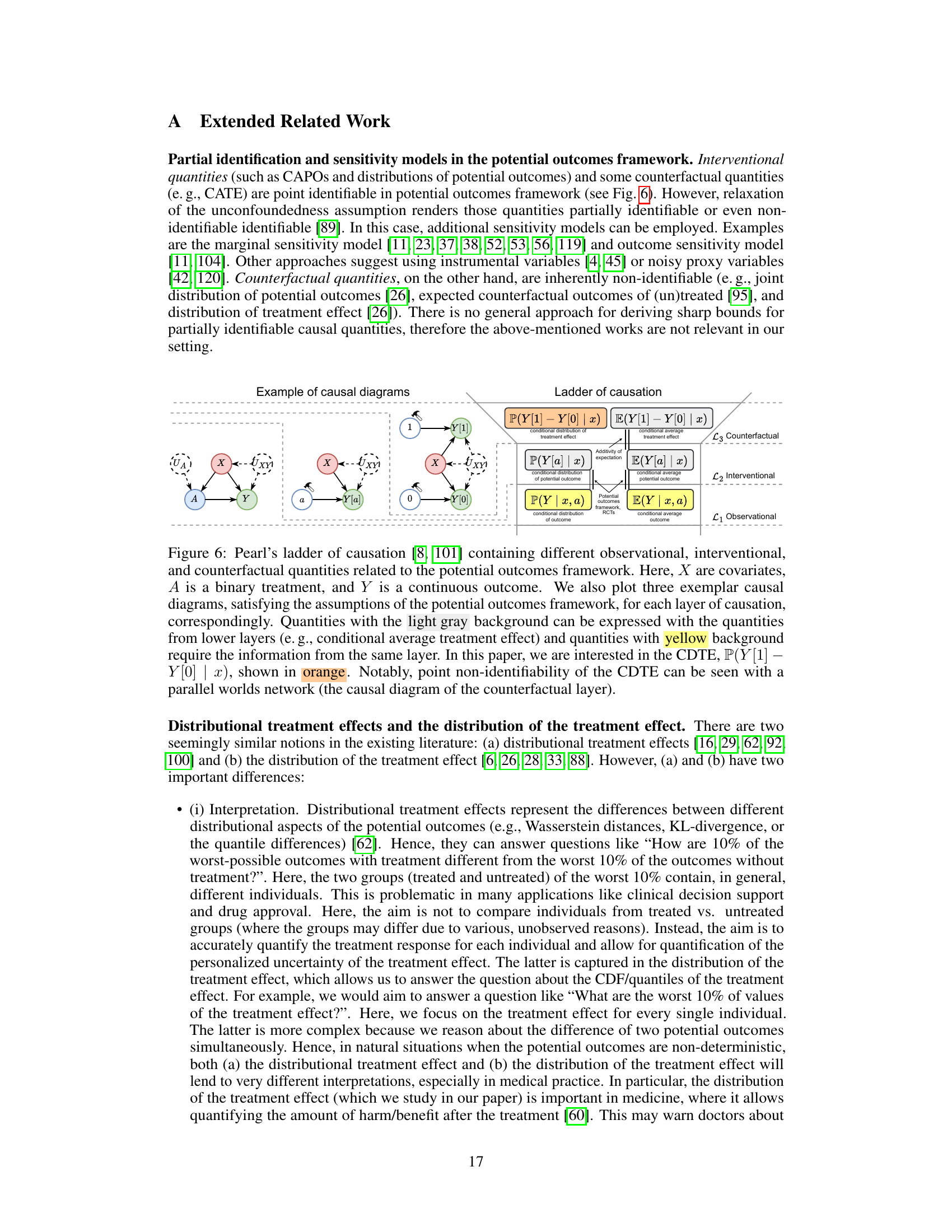
This figure compares and contrasts the identification and estimation processes for Conditional Average Treatment Effect (CATE) and Conditional Distribution of Treatment Effects (CDTE). It highlights the key differences in identifiability (CATE is point-identifiable, CDTE is not), the form of the target estimand (closed-form for CATE, no closed-form for CDTE), and the constraints on the target estimand (unconstrained for CATE, bounded by Makarov bounds for CDTE). The figure visually represents these differences and illustrates the paper’s main contribution: a novel orthogonal learner for estimating the CDTE.

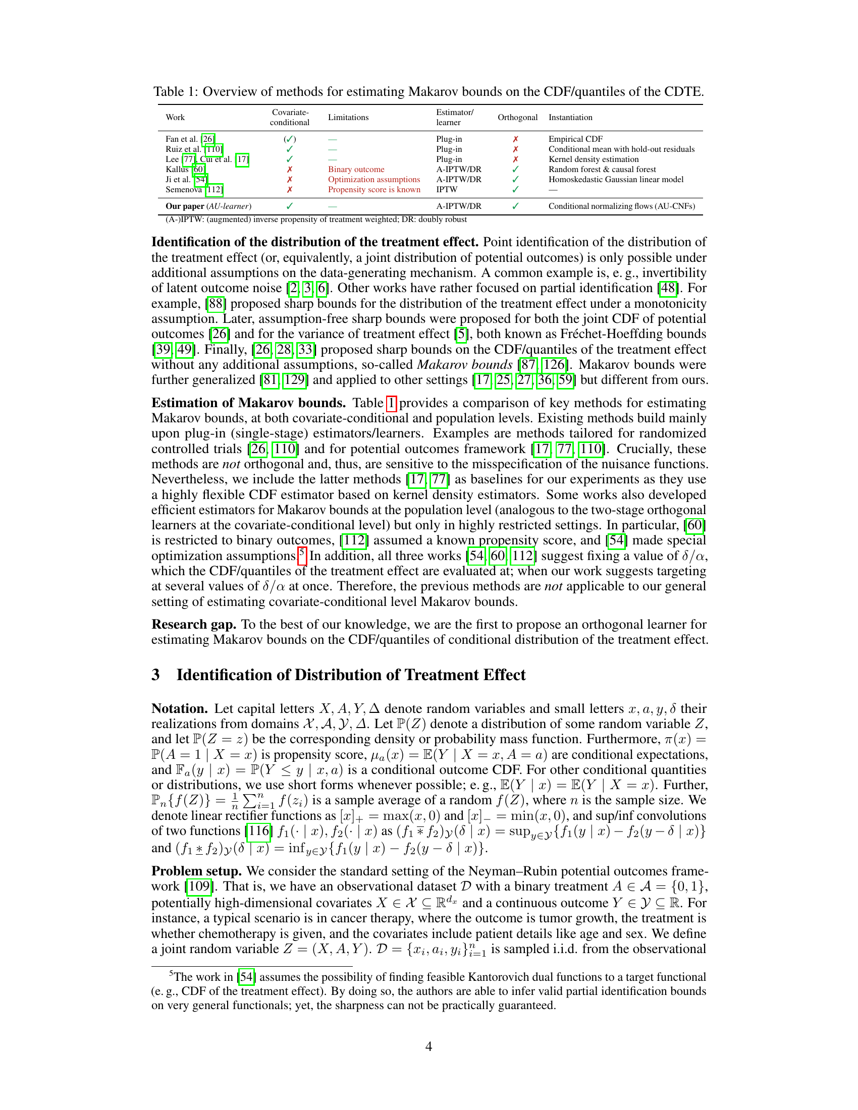
The table provides a comparison of key methods for estimating Makarov bounds on the cumulative distribution function (CDF) and quantiles of the conditional distribution of the treatment effect (CDTE). It compares various methods based on their characteristics, including whether they are covariate-conditional, whether they use orthogonal learners, and any limitations they have. The table highlights the novelty of the AU-learner proposed in the paper, which addresses limitations present in previous methods.
In-depth insights#
Aleatoric Uncertainty#
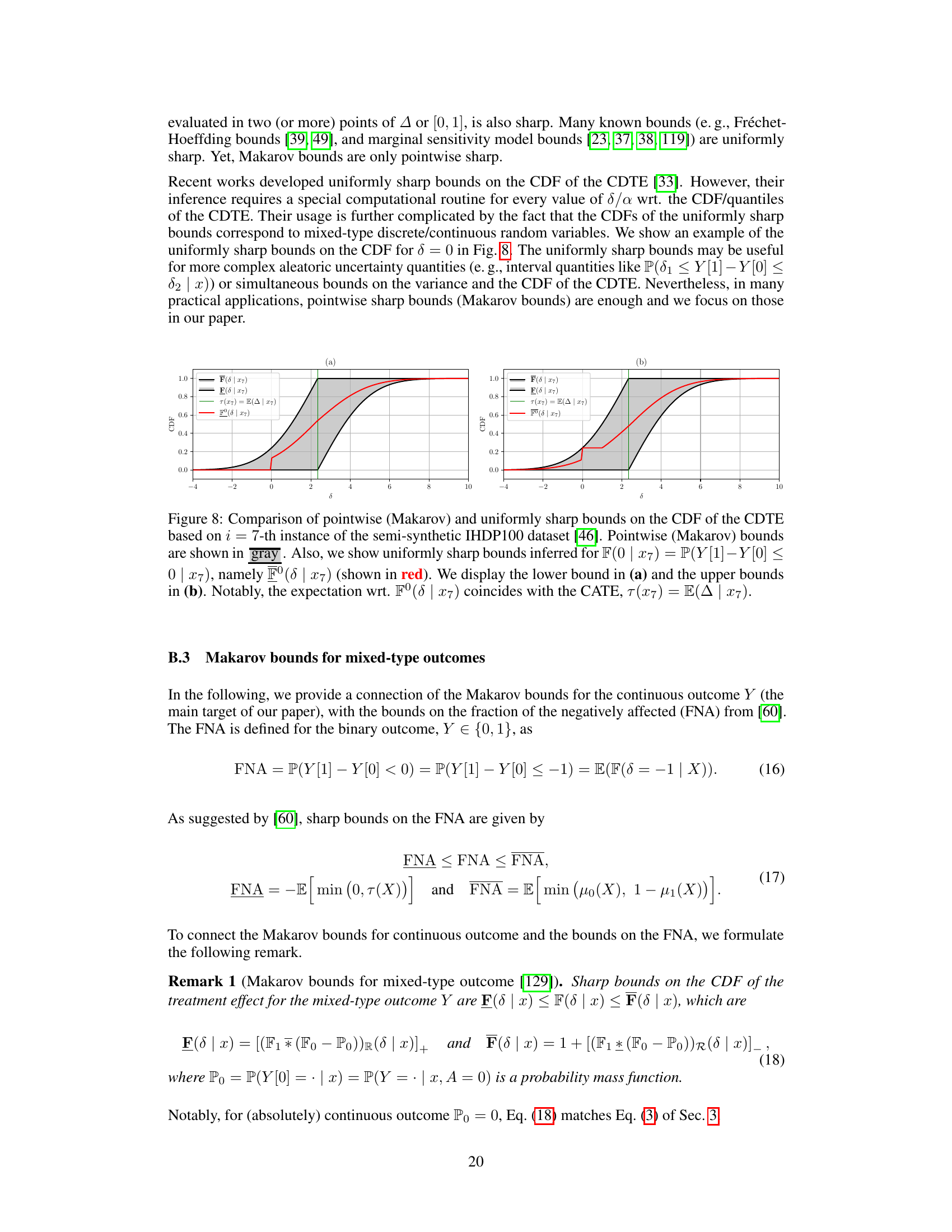
Aleatoric uncertainty, inherent randomness in data, is a critical concept when assessing treatment effects. Standard methods often focus solely on average treatment effects (ATEs), neglecting the inherent variability. This is problematic as individuals respond differently. Quantifying aleatoric uncertainty allows for a deeper understanding of treatment effect distributions, enabling the calculation of probabilities of benefit, quantiles, and variance at both population and covariate-conditional levels. Challenges in quantifying this uncertainty include the non-point identifiability of the conditional distribution of treatment effects (CDTE), requiring partial identification methods. This necessitates novel orthogonal learners, like the AU-learner, which offer robustness and efficiency. The AU-learner addresses the challenges of estimating Makarov bounds by leveraging partial identification and ensuring Neyman-orthogonality, thus providing a more complete and reliable picture of treatment effectiveness. Further research could explore extensions to handle different outcome types and further enhance the AU-learner’s performance in low-sample scenarios.
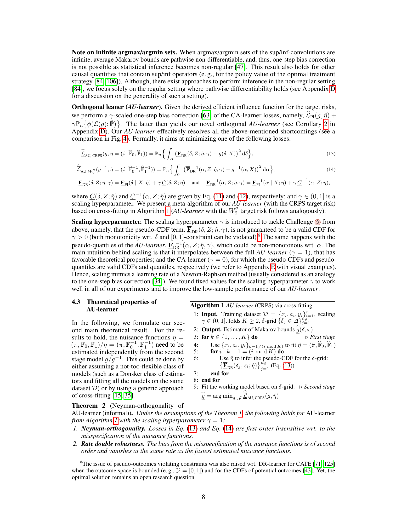
Orthogonal AU-learner#
The heading “Orthogonal AU-learner” suggests a novel machine learning algorithm designed for causal inference, specifically targeting the quantification of aleatoric uncertainty in treatment effects. The “AU” likely refers to “Aleatoric Uncertainty,” representing the inherent randomness in the treatment effect. Orthogonality is a crucial aspect, implying the algorithm’s robustness against biases from misspecified nuisance functions (e.g., propensity scores). This characteristic is highly desirable in causal inference because it reduces sensitivity to modeling errors, improving the reliability of estimates. The combination of both suggests a method that is not only accurate in estimating the conditional distribution of treatment effects but also statistically efficient and less prone to errors, a significant advantage over previous plug-in methods. This approach’s strength likely lies in its theoretical guarantees and improved performance in low-sample settings where simpler approaches suffer from high variance and unreliable results.
Makarov Bounds#
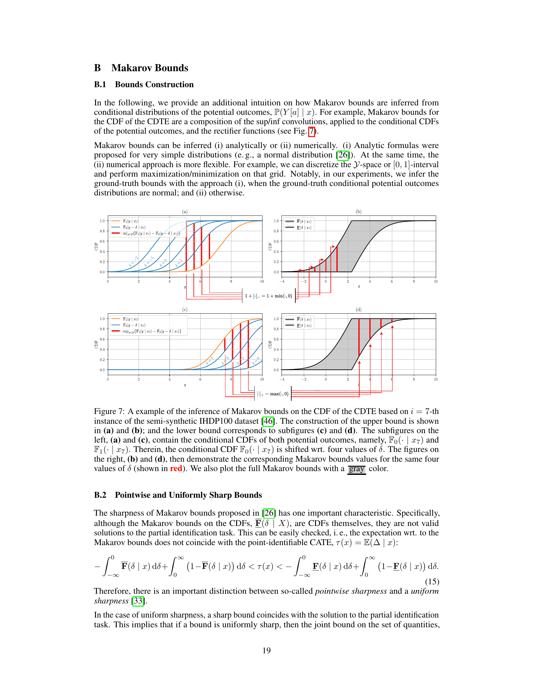
Makarov bounds offer a powerful yet often overlooked method for addressing the challenges of causal inference, specifically when dealing with the conditional distribution of the treatment effect (CDTE). Unlike traditional average treatment effect (ATE) estimations, which focus on the mean, Makarov bounds provide sharp, assumption-free bounds on the cumulative distribution function (CDF) and quantiles of the CDTE. This approach is particularly valuable when point identification is not possible due to inherent limitations in observational data. Partial identification, the foundation of Makarov bounds, acknowledges the limitations imposed by unobserved counterfactuals, making it a robust and reliable approach. The methodology leverages the sup/inf convolutions of conditional CDFs for potential outcomes to construct informative bounds, capturing the inherent aleatoric uncertainty. While the bounds may not be point estimates, they provide crucial insights into the potential range of treatment effects under specific conditions, enhancing the reliability of causal analysis and improving decision making. The bounds’ monotonicity, though a constraint, ensures useful information even without perfect identification. The development of efficient and orthogonal learners for estimating Makarov bounds is crucial for practical applications, which is an active area of ongoing research. The strength lies in the robustness provided by acknowledging and incorporating the inherent uncertainties involved in causal estimation. In short, while not delivering point estimates, Makarov bounds provide a crucial framework for reliable causal inference in scenarios with inherent uncertainty and unobservable counterfactuals.
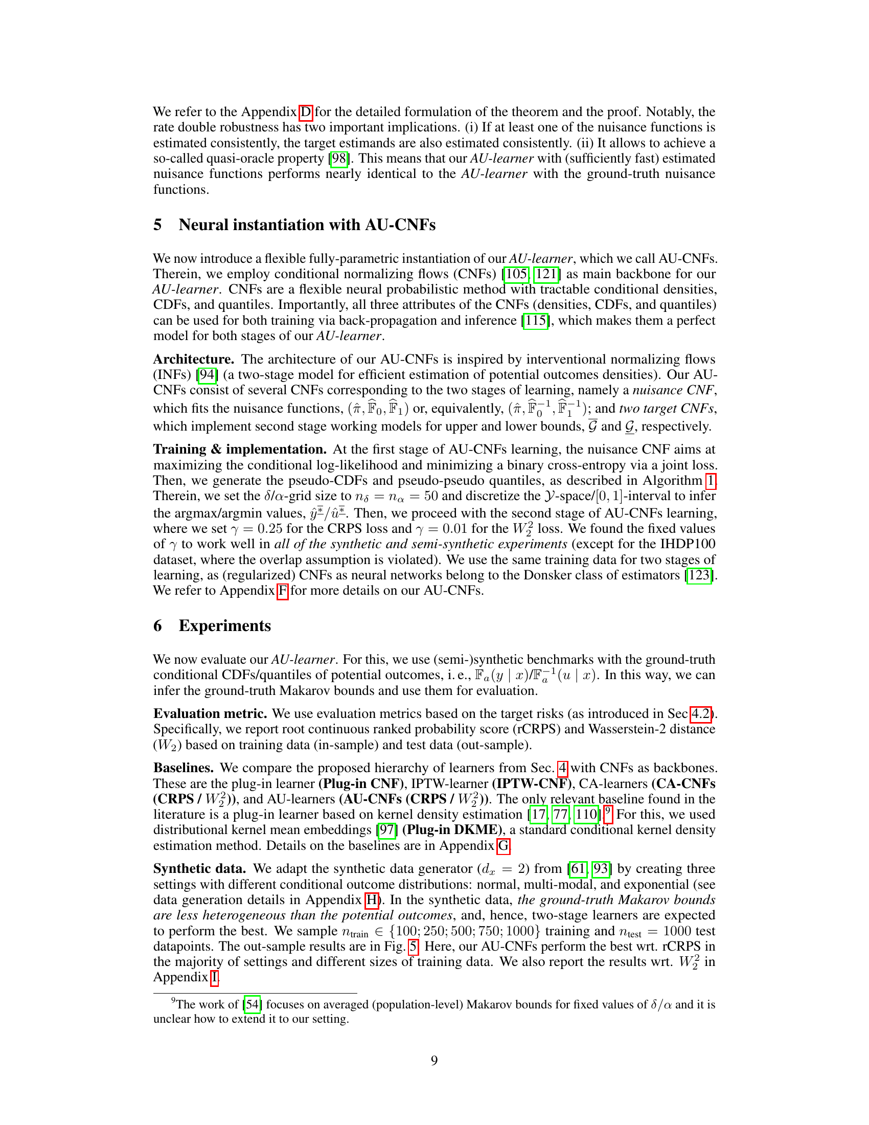
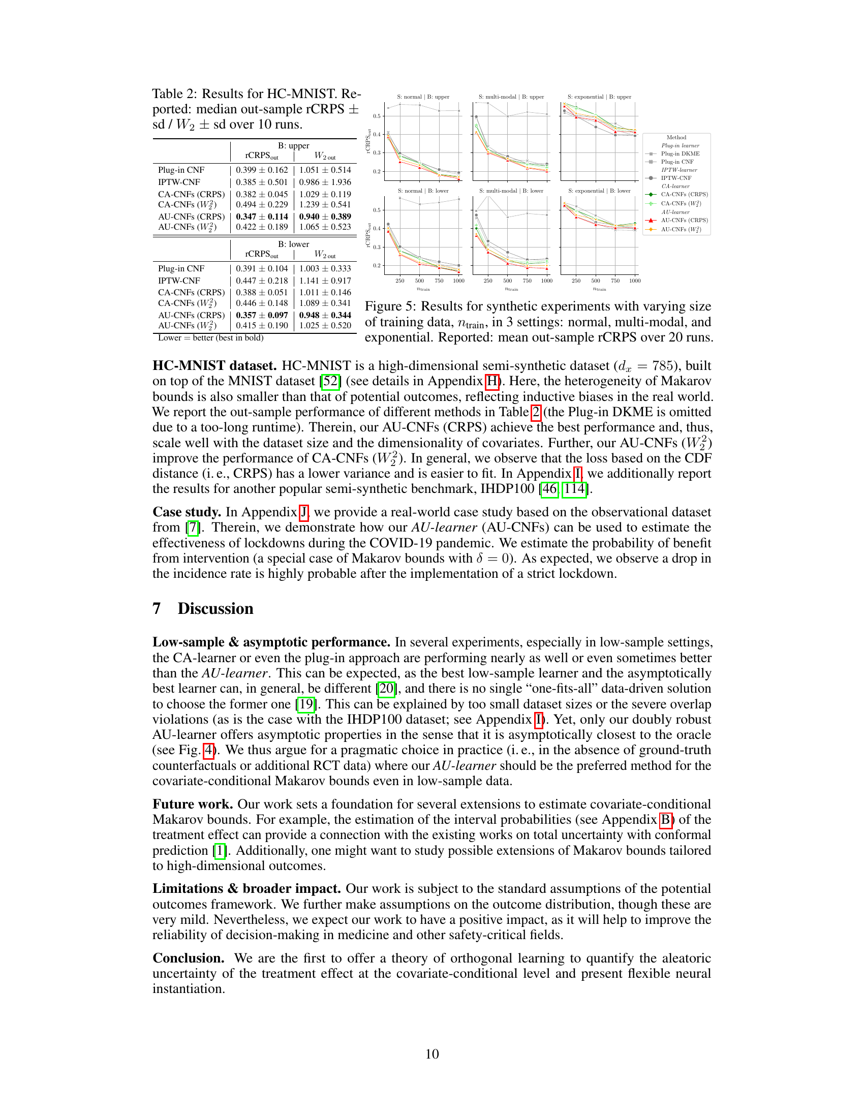
AU-CNF Instantiation#
The AU-CNF instantiation section likely details a practical implementation of the AU-learner algorithm using Conditional Normalizing Flows (CNFs). CNFs are chosen for their ability to model complex probability distributions and efficiently estimate both densities and quantiles, aligning well with the need to estimate Makarov bounds. The instantiation would involve specifying the architecture of the CNF, including the number of layers and the type of flow used, along with the specific loss function employed for optimization. The authors likely address training procedures, specifying the training process and hyperparameters for the CNF, and compare the performance of the AU-CNF to alternative estimators, possibly using standard benchmark datasets. Importantly, the evaluation likely focuses on the AU-CNF’s ability to accurately estimate Makarov bounds, considering both the sharpness and coverage of the estimated bounds. Finally, this section might include an analysis of the AU-CNF’s computational efficiency and scalability, a crucial aspect for real-world applications of causal inference.
Future Work#
The “Future Work” section of a research paper on quantifying aleatoric uncertainty in treatment effects using a novel orthogonal learner (AU-learner) would naturally explore several avenues. Extending the AU-learner to handle high-dimensional outcomes is a crucial direction, as real-world datasets often involve complex, multi-faceted outcomes beyond simple continuous variables. Investigating the performance of the AU-learner under various assumptions such as the strength of unconfoundedness and overlap is essential to better understand its robustness. Furthermore, a comparison to other methods for quantifying distributional treatment effects within a unified framework is needed, especially for scenarios where the AU-learner’s strong assumptions are relaxed. Developing more efficient deep learning implementations may also enhance the AU-learner’s applicability to larger datasets, as computational cost can be a significant barrier in practice. Finally, exploring applications to specific real-world problems, including those with significant ethical considerations, offers a path to demonstrating the method’s practical value and addressing critical questions within healthcare or similar domains.
More visual insights#
More on figures
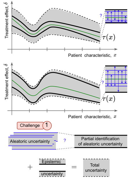
This figure compares the identification and estimation of the conditional average treatment effect (CATE) with the conditional distribution of the treatment effect (CDTE). It highlights the challenges in estimating the CDTE, such as its non-point identifiability, lack of closed-form expression, and constrained nature compared to the unconstrained CATE. The figure shows that the authors’ main contribution is a novel method to estimate the cumulative distribution function (CDF) of the CDTE, addressing these challenges.
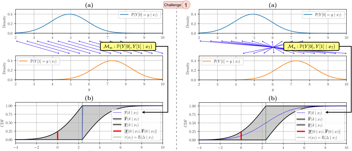
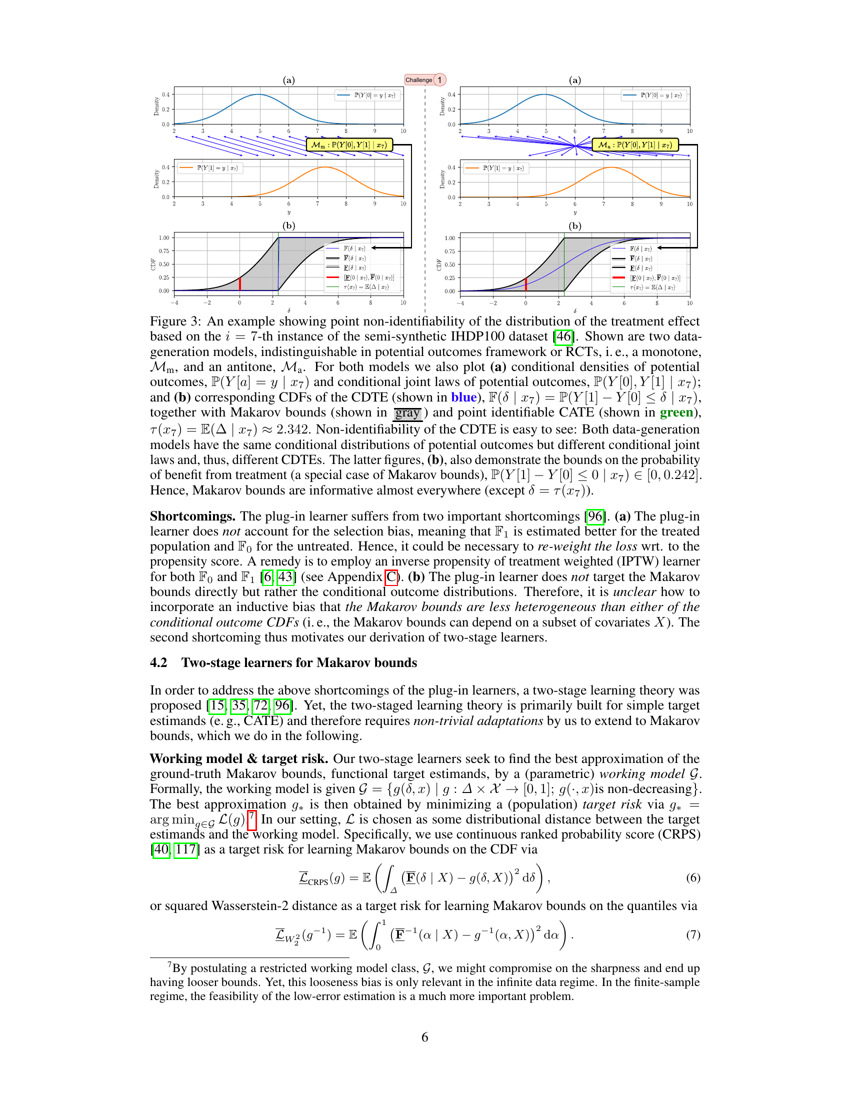
This figure shows an example demonstrating the non-identifiability of the distribution of the treatment effect using the IHDP100 dataset. It compares two data-generating models (monotone and antitone) which produce identical conditional distributions of potential outcomes but different conditional distributions of treatment effects (CDTE). The figure highlights the Makarov bounds, which provide partial identification of the CDTE, in contrast to the point-identifiable conditional average treatment effect (CATE). A key takeaway is that, even with identical observable distributions, the underlying CDTE may differ.

This figure compares four different learners for estimating Makarov bounds: the plug-in learner, the IPTW-learner, the CA-learner, and the AU-learner. It highlights the key differences between the learners in terms of addressing selection bias, directly targeting Makarov bounds, and achieving orthogonality of the loss with respect to the nuisance functions. The AU-learner, proposed by the authors, is shown to be superior to the other methods by addressing all three aspects.

This figure compares and contrasts the identification and estimation processes for Conditional Average Treatment Effect (CATE) and Conditional Distribution of Treatment Effect (CDTE). It highlights the key differences and challenges involved in estimating CDTE, such as its non-point identifiability, lack of closed-form expression, and constrained nature compared to CATE.

This figure compares and contrasts the identification and estimation of the conditional average treatment effect (CATE) with the conditional distribution of the treatment effect (CDTE). It highlights the challenges in estimating the CDTE, which include its non-point identifiability, lack of a closed-form expression, and constrained nature (Makarov bounds) compared to the unconstrained CATE. The figure visually represents these concepts using different colors to represent different aspects of the process and emphasizes the paper’s contribution focuses on estimating the CDF of the CDTE.

This figure compares the identification and estimation processes for Conditional Average Treatment Effect (CATE) and Conditional Distribution of Treatment Effects (CDTE). It highlights the key differences and challenges in moving from the well-studied CATE estimation to the novel CDTE estimation proposed in the paper. The figure illustrates that while CATE is point identifiable, CDTE is not, requiring partial identification methods. It also shows that the CDTE lacks a closed-form expression, preventing direct adaptation of CATE learners. Finally, it emphasizes that CATE is an unconstrained target, while CDTE is constrained by Makarov bounds.

This figure demonstrates the non-identifiability of the Conditional Distribution of Treatment Effects (CDTE) using the IHDP100 dataset. It compares two data-generating models (monotone and antitone) that produce identical conditional average treatment effects (CATE) but different CDTEs. The figure highlights the CDTE’s CDF, Makarov bounds (providing sharp bounds for the CDTE), and the CATE, illustrating how the CDTE cannot be point identified without strong additional assumptions. A key takeaway is the non-identifiability despite identical CATEs.
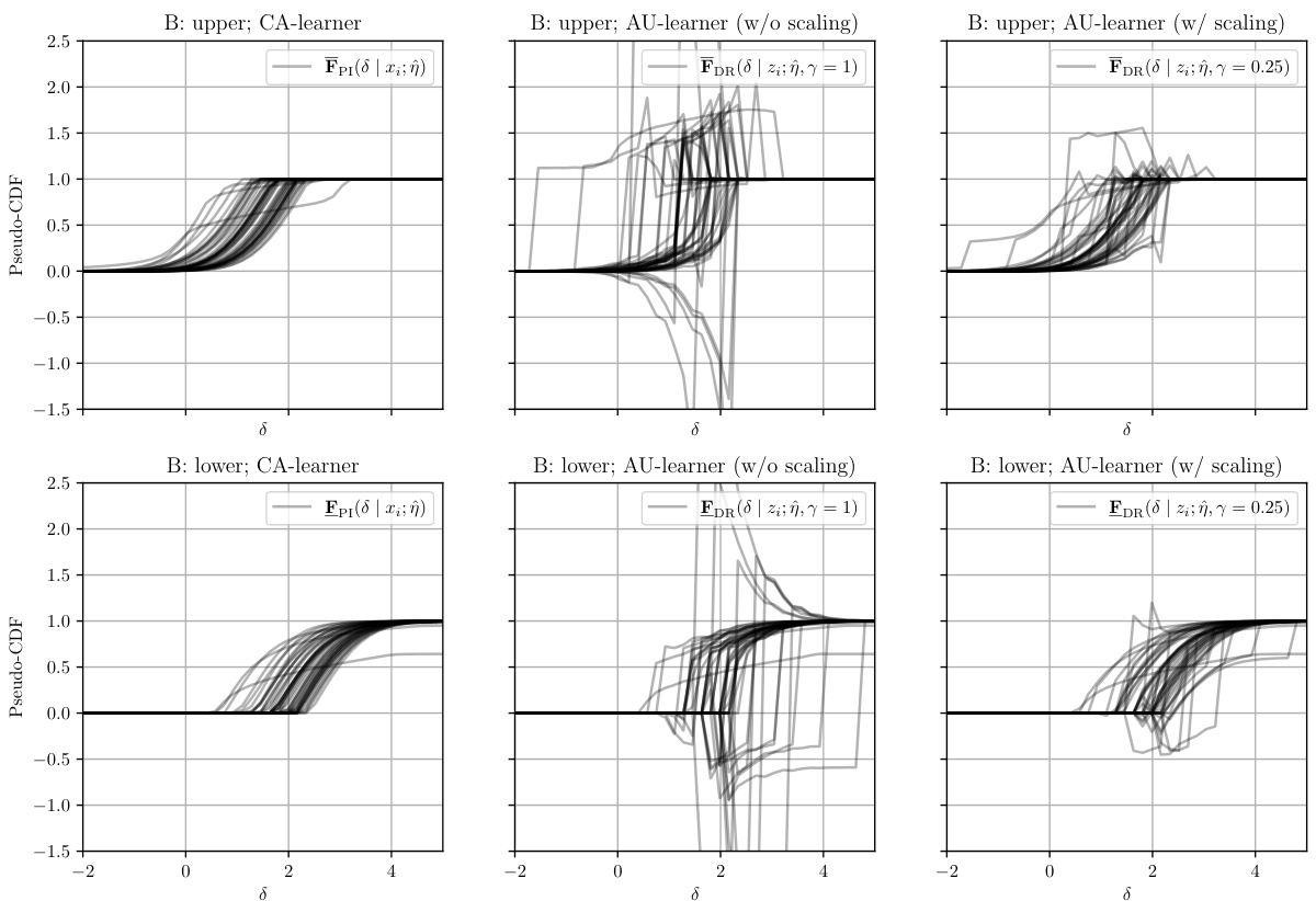
This figure compares the identification and estimation processes for Conditional Average Treatment Effect (CATE) and Conditional Distribution of Treatment Effect (CDTE). It highlights the key differences and challenges in estimating CDTE, such as its non-point identifiability, lack of closed-form expression, and the constrained nature of Makarov bounds (used to address the non-identifiability) compared to the simpler CATE.

This figure compares and contrasts the identification and estimation of the conditional average treatment effect (CATE) with the conditional distribution of the treatment effect (CDTE). It highlights the challenges in estimating the CDTE, such as its non-point identifiability, lack of a closed-form expression, and constrained nature compared to the unconstrained CATE. The figure visually represents the different methods and challenges involved in estimating both quantities.

This figure demonstrates the point non-identifiability of the conditional distribution of the treatment effect (CDTE). It shows two data-generating processes that produce the same conditional distributions of potential outcomes but different CDTEs, highlighting the challenge in estimating the CDTE. Makarov bounds and the conditional average treatment effect (CATE) are also shown for comparison.
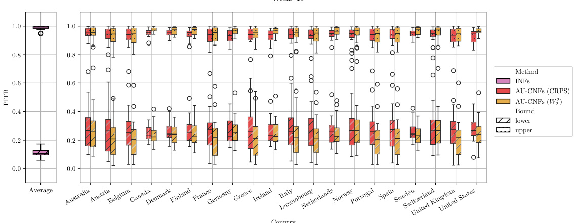
This figure illustrates the non-identifiability of the conditional distribution of the treatment effect (CDTE). It compares two data-generating models (monotone and antitone) that produce indistinguishable results in randomized controlled trials (RCTs) or the standard potential outcomes framework. However, these models yield different conditional distributions for the treatment effect despite having identical conditional distributions for potential outcomes. The figure highlights the Makarov bounds, which provide sharp bounds on the CDTE, illustrating how partial identification can be used to quantify aleatoric uncertainty.
More on tables
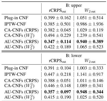
This table compares various methods for estimating Makarov bounds on the cumulative distribution function (CDF) and quantiles of the Conditional Distribution of the Treatment Effect (CDTE). It contrasts methods based on plug-in estimators with those using augmented inverse propensity of treatment weighted (A-IPTW) or doubly robust (DR) approaches, highlighting their strengths and limitations regarding covariate conditioning, orthogonality, and the types of estimators used. The table shows that the proposed AU-learner method from the paper is unique in its ability to be both covariate-conditional and orthogonal, offering improvements over existing approaches.
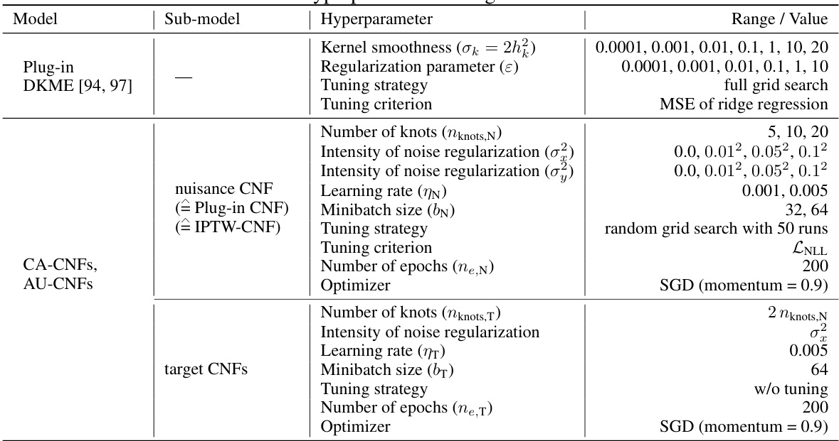
This table compares different methods for estimating Makarov bounds on the cumulative distribution function (CDF) and quantiles of the conditional distribution of the treatment effect (CDTE). It highlights whether each method is covariate-conditional, uses an orthogonal learner, and lists any limitations. The methods include plug-in estimators, inverse propensity of treatment weighted (IPTW) learners, and doubly robust (DR) learners. The table serves as a benchmark for the novel AU-learner proposed in the paper.
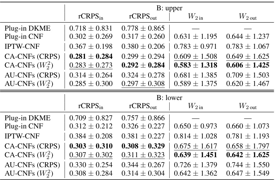
This table compares different methods for estimating Makarov bounds on the cumulative distribution function (CDF) and quantiles of the conditional distribution of the treatment effect (CDTE). It shows existing methods, highlighting their limitations such as being restricted to binary outcomes, needing prior knowledge of propensity scores, or making strong optimization assumptions. The table also points out whether a method is covariate-conditional (meaning it estimates the bounds based on individual patient characteristics) and uses an orthogonal learner for estimation. Finally, it compares these to the new method proposed in the paper (AU-learner), highlighting its advantages.

This table compares existing methods for estimating Makarov bounds on the cumulative distribution function (CDF) and quantiles of the conditional distribution of the treatment effect (CDTE). It highlights whether methods are covariate-conditional, use orthogonal learners, and their limitations. The table helps contextualize the AU-learner proposed in the paper by showing its advantages over existing approaches.
Full paper#
