↗ OpenReview ↗ NeurIPS Homepage ↗ Chat
TL;DR#
Causal discovery, determining cause-and-effect relationships, often relies on interventional data – experiments altering variables. However, these experiments can be costly and limited. Existing methods usually assume perfect or unlimited interventions, a major limitation. This research directly addresses this problem.
The proposed solution leverages a Bayesian approach with a focus on efficiently tracking the posteriors of various interventional scenarios. By using a smart algorithm for uniformly sampling directed acyclic graphs (DAGs), the method accurately infers causal structures even with limited interventions. This innovative approach has been rigorously tested against existing methods, demonstrating superior accuracy and efficiency in various simulated datasets. It’s also adaptable to answering broader causal questions without needing to build the entire causal graph.
Key Takeaways#
Why does it matter?#
This paper is crucial because it tackles the challenge of causal discovery with limited interventional data, a common constraint in real-world applications. It offers a novel Bayesian approach that significantly improves accuracy and efficiency, reducing the number of interventions needed compared to existing methods. This opens up new possibilities for various fields where interventions are expensive or difficult to perform.
Visual Insights#
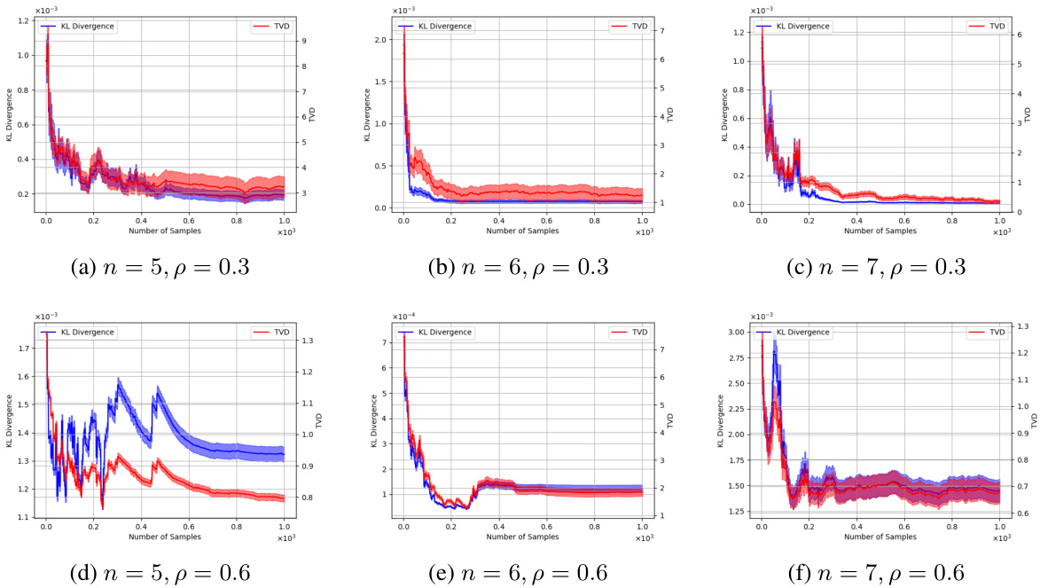
This figure shows the results of an experiment to evaluate the accuracy of estimating causal effects using the proposed Bayesian approach. The experiment used random causal graphs with varying numbers of nodes (n=5, 6, 7) and densities (p=0.3, 0.6). For each graph and density, multiple trials were performed, each with a varying number of interventional samples. The plot shows the average KL divergence and Total Variation Distance (TVD) between the estimated causal effect and the ground truth. The shaded regions represent the standard deviation across multiple trials. The results demonstrate that as the number of interventional samples increases, both the KL divergence and TVD decrease, indicating improved accuracy in estimating causal effects.
This figure compares the performance of the proposed algorithm against two other Bayesian causal discovery methods (scm-v0 and neurips-rff) on random complete graphs. The Structural Hamming Distance (SHD), a measure of the difference between learned and true causal graphs, is plotted against the number of interventional samples. The average SHD and standard deviation across 50 random DAGs are shown.
In-depth insights#
Bayesian Causal Discovery#
Bayesian causal discovery leverages the power of Bayesian inference to uncover causal relationships from data. Unlike frequentist approaches, it directly models uncertainty about the causal graph structure using probability distributions over the space of possible Directed Acyclic Graphs (DAGs). This allows for a more nuanced representation of causal knowledge, incorporating both observational and interventional data. The Bayesian framework facilitates the incorporation of prior knowledge about the system, improving efficiency and robustness, especially with limited data. Markov Chain Monte Carlo (MCMC) methods are commonly used to sample from the posterior distribution over DAGs, allowing for inference about the most likely causal structure and the strength of causal effects. Challenges include the computational complexity of exploring the space of DAGs and the sensitivity to prior assumptions. However, advances in MCMC algorithms and the development of efficient DAG samplers are continually addressing these issues, making Bayesian causal discovery a powerful tool for causal inference in various scientific fields.
Intervention Strategies#
Intervention strategies in causal discovery research are crucial for reliably disentangling cause-and-effect relationships. Optimal strategies aim to minimize the number of interventions while maximizing information gained, often employing adaptive designs that select future interventions based on results from previous ones. Adaptive methods are particularly valuable when interventions are costly or risky. Non-adaptive methods, in contrast, plan all interventions beforehand, which allows for parallelization but may require more interventions overall. A key challenge lies in balancing exploration (learning about the causal structure) and exploitation (confirming existing knowledge). Bayesian approaches offer a robust framework by incorporating prior knowledge and quantifying uncertainty in the learned causal graph, enabling efficient decision-making under limited data. There is ongoing research focusing on the development of more efficient and adaptive intervention strategies, particularly in settings with constraints on the types or feasibility of interventions. Careful consideration of cost and feasibility is paramount, as is addressing potential ethical implications related to performing interventions.
Limited Data Learning#
The concept of ‘Limited Data Learning’ in the context of causal discovery is critical due to the often high cost and difficulty of obtaining interventional data. Traditional methods assume abundant data, which is unrealistic in many real-world scenarios. Therefore, research in this area focuses on developing algorithms robust to scarce interventional data. This involves using Bayesian approaches to effectively quantify uncertainty inherent in limited samples, leveraging prior knowledge or assumptions to guide learning, and employing techniques for efficient exploration of the causal space with limited interventions. Bayesian methods, for example, can incorporate prior beliefs and update posterior probabilities as new data arrive, allowing for more accurate estimations with fewer interventions. Adaptive methods iteratively choose interventions based on previously gathered information to maximize learning efficiency. The core challenge, and active research area, lies in designing these algorithms to achieve accurate and reliable causal graph estimation even with noisy and incomplete data. Theoretical analysis, proving guarantees on correctness, is also vital to understand the capabilities and limitations under various conditions.
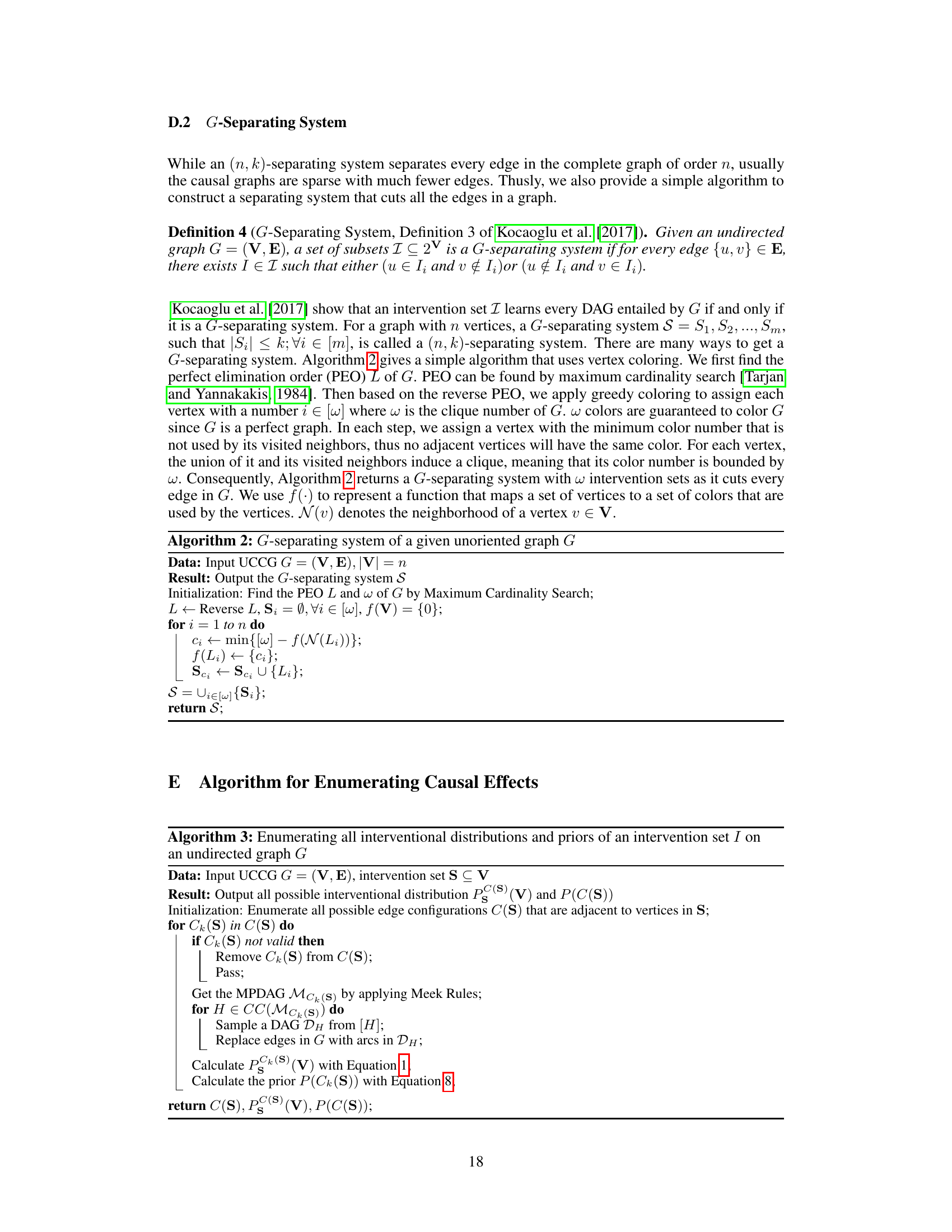
Algorithm Analysis#
A thorough algorithm analysis is crucial for evaluating a research paper. It should delve into the algorithm’s correctness, proving that it produces the desired output under specified conditions. Time complexity analysis, using Big O notation, assesses how the runtime scales with input size. Space complexity analysis examines memory usage. The analysis should also discuss the algorithm’s robustness to noisy or incomplete data and its scalability to large datasets. Comparative analysis against existing methods is vital, highlighting improvements in efficiency or accuracy. Finally, a discussion on practical considerations like implementation details and potential bottlenecks is necessary for a complete evaluation.
Causal Effect Estimation#
Causal effect estimation, a critical aspect of causal inference, seeks to quantify the impact of one variable on another, isolating the true causal relationship from confounding factors. Accurate estimation requires careful consideration of confounding variables, often using techniques such as regression adjustment or propensity score matching. The choice of method depends heavily on the nature of the data and the specific research question. Assumptions underlying causal effect estimation, such as the ignorability assumption (no unmeasured confounding), are crucial and should be critically evaluated. The presence of unobserved confounders can lead to biased estimates, highlighting the importance of robust identification strategies and sensitivity analyses. Advances in causal discovery, such as those leveraging interventional data, offer new possibilities for improving the accuracy of causal effect estimations. Furthermore, the development of more flexible methods that can accommodate different data types and handle complex relationships remains an active area of research.
More visual insights#
More on figures

This figure compares the performance of four causal discovery algorithms (Active Learning using DCT, Random Intervention, Adaptivity-sensitive Search, and the proposed algorithm) on complete graphs with varying numbers of nodes (n=5, 6, and 7). The x-axis represents the number of interventional samples used, and the y-axis shows the Structural Hamming Distance (SHD), a measure of the difference between the learned causal graph and the true graph. Lower SHD indicates better performance. The figure demonstrates that the proposed algorithm consistently achieves lower SHD with fewer interventional samples compared to the baselines, indicating its superior sample efficiency.

This figure compares the performance of four causal discovery algorithms (Active Learning using DCT, Random Intervention, Adaptivity-sensitive Search, and the proposed algorithm) on complete graphs with varying sizes (n=5, 6, 7). The x-axis represents the number of interventional samples, while the y-axis shows the Structural Hamming Distance (SHD) between the learned causal graph and the ground truth. Lower SHD values indicate better performance. The shaded area represents the standard deviation. The figure demonstrates the superior performance of the proposed algorithm, particularly in requiring fewer interventional samples to achieve a low SHD.

This figure displays the results of an experiment comparing the performance of the proposed algorithm in estimating causal effects against the ground truth. Two metrics are used: Kullback-Leibler (KL) divergence and Total Variation Distance (TVD). The x-axis represents the number of interventional samples used, and the y-axis shows the average divergence (KL and TVD) between the estimated causal effect and the true causal effect. Multiple graphs are shown, each representing different settings (number of vertices and density) in randomly generated causal graphs.

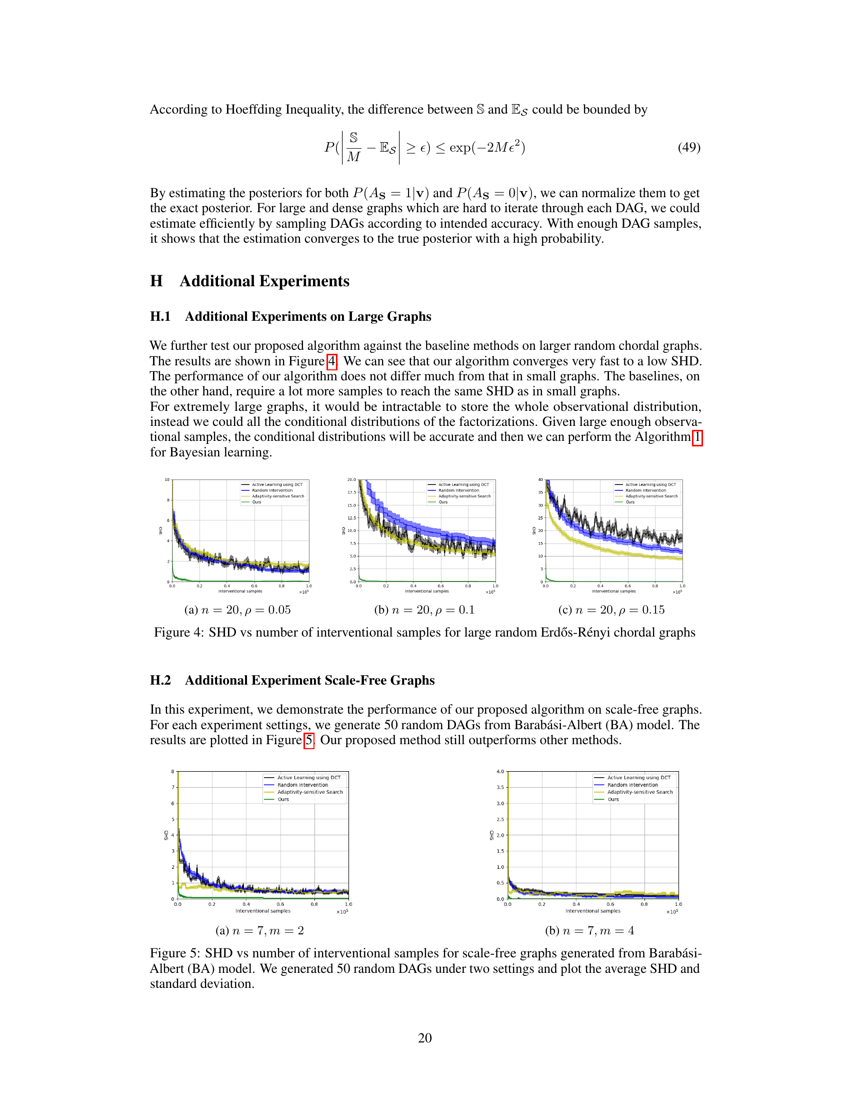
The figure shows the Structural Hamming Distance (SHD) between the estimated causal graph and the ground truth plotted against the number of interventional samples for large random Erdős-Rényi chordal graphs with different densities (p = 0.05, 0.1, 0.15). It compares the performance of the proposed Bayesian Causal Discovery algorithm with three baselines: Active Learning using DCT, Random Intervention, and Adaptivity-sensitive Search. The results demonstrate that the proposed algorithm converges faster to a lower SHD than the baseline methods, especially as the density of the graph increases.

This figure compares the performance of the proposed Bayesian causal discovery algorithm against three baseline methods on scale-free graphs generated using the Barabási-Albert model. The y-axis represents the Structural Hamming Distance (SHD), a metric measuring the difference between the learned causal graph and the true graph. The x-axis shows the number of interventional samples used. The figure plots the average SHD and its standard deviation across 50 different scale-free graph instances for two distinct parameter settings (n=7, m=2 and n=7, m=4; where n is the number of nodes and m is a parameter of the BA model affecting the scale-free property). The results demonstrate that the proposed algorithm achieves lower SHD with fewer interventional samples compared to the baseline methods.

This figure compares the performance of the proposed Bayesian causal discovery algorithm against two existing Bayesian algorithms (scm-v0 and neurips-rff) on random complete graphs. The Structural Hamming Distance (SHD), a measure of the difference between the learned causal graph and the true causal graph, is plotted against the number of interventional samples used. The plot shows that the proposed algorithm achieves significantly lower SHD with fewer interventional samples compared to the two baselines.
Full paper#
