↗ OpenReview ↗ NeurIPS Homepage ↗ Hugging Face ↗ Chat
TL;DR#
Scaling up neural networks is crucial for progress in deep learning, but it poses a challenge: hyperparameter tuning becomes increasingly expensive and time-consuming as models grow larger. This paper addresses this issue by exploring how some hyperparameters, such as the learning rate, can be transferred from small to very large models. Previous research highlighted that such transfer is puzzling, suggesting the loss landscape remains similar across vastly different model sizes.
This research investigates this phenomenon through a novel concept: “Super Consistency.” This property highlights the consistency of certain spectral properties of the loss landscape (specifically, its largest eigenvalue or ‘sharpness’) across various model sizes, regardless of the network’s size. The authors show that this Super Consistency is strongly linked to the ability to transfer hyperparameters, specifically the learning rate. They found this property holds for feature-learning parameterizations (like µP) but not others (like NTK), indicating a strong link between feature learning and this property.
Key Takeaways#
Why does it matter?#
This paper is crucial for researchers working with large neural networks. It addresses the significant challenge of hyperparameter tuning in massive models by identifying a key property, Super Consistency, which explains the transferability of learning rates across vastly different model sizes. This is important because it offers a solution to the expensive and time-consuming process of hyperparameter tuning for large models, and opens up new research directions in optimization and scaling limits.
Visual Insights#

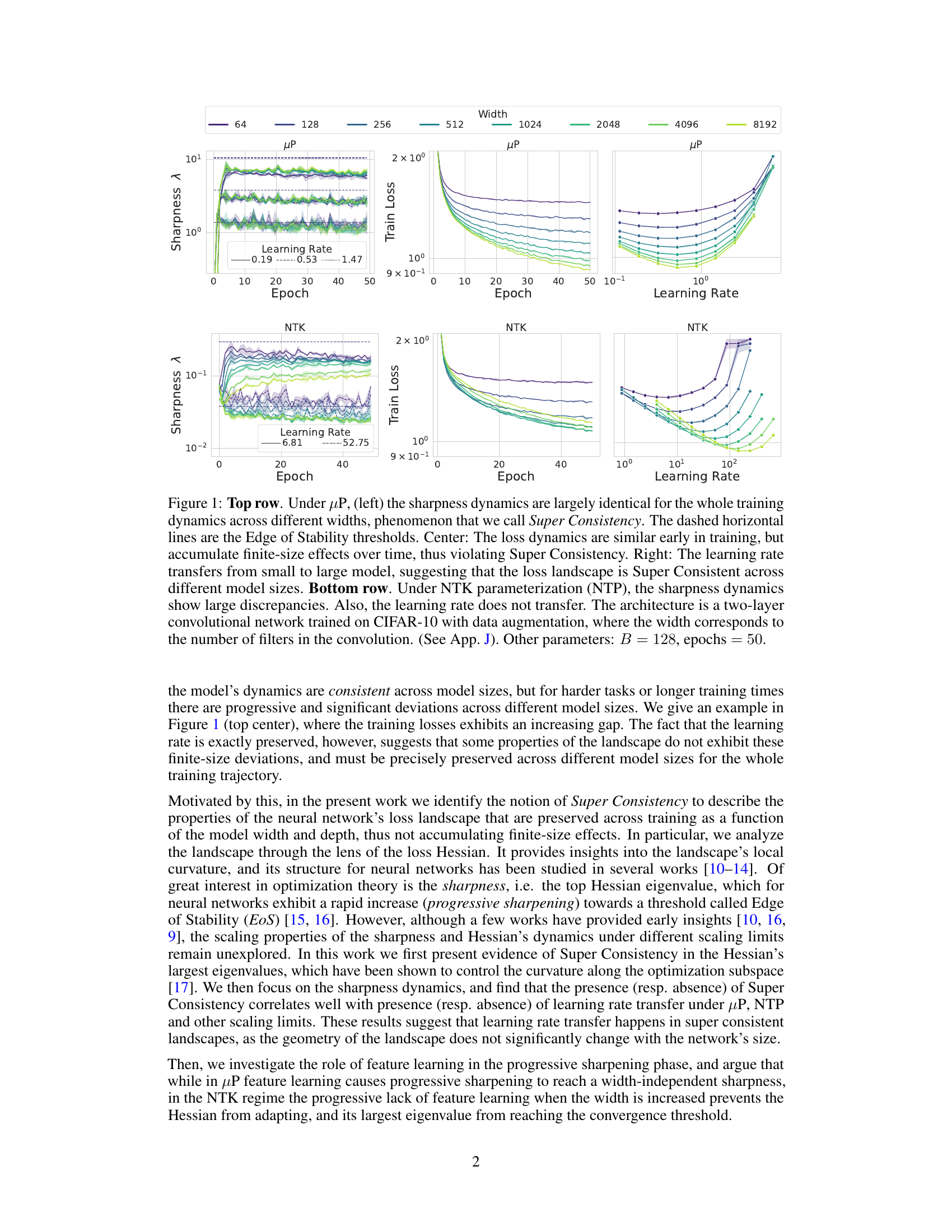
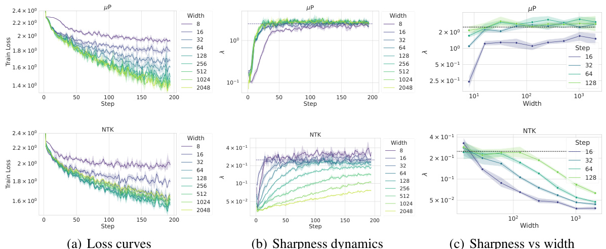
The figure shows the training dynamics of sharpness and loss under two different parameterizations, µP and NTK. Under µP scaling, sharpness remains consistent across different network widths, a phenomenon termed ‘Super Consistency.’ The loss curves show slight differences at later stages. Importantly, the learning rate transfers successfully from smaller to larger models under µP. In contrast, under NTK parameterization, sharpness dynamics differ significantly across widths, and learning rate transfer fails. The experiment is performed on a two-layer convolutional network trained on CIFAR-10.

This table summarizes the scaling of different hyperparameters for various neural network parametrizations. It shows how the learning rate (η), output multiplier (γ), and depth-scaling exponents (α) are adjusted for different methods (SGD and Adam) with and without residual connections. The table highlights the µP parametrization as a special case of Depth-µP where depth dependence is ignored. Note that for Adam, the epsilon parameter is set to zero.
In-depth insights#
Hessian SuperConsistency#
The concept of “Hessian SuperConsistency” centers on the observation that specific spectral properties of the loss Hessian remain remarkably consistent across different neural network sizes during training. This consistency, particularly regarding the largest eigenvalue (sharpness), is surprisingly independent of model width and depth. This phenomenon is intriguing because it implies a degree of universality in the optimization landscape, facilitating the transfer of hyperparameters (like learning rate) between models of vastly different scales. The study connects Hessian SuperConsistency to the presence or absence of effective feature learning during training. Regimes exhibiting this property show consistent sharpness dynamics and learning rate transfer, while regimes lacking it do not. Ultimately, the research suggests that Hessian SuperConsistency is a crucial factor explaining the successful transfer of hyperparameters in deep learning, highlighting the importance of feature learning in shaping the optimization landscape and ensuring consistent training dynamics across various scales.
Feature Learning Effects#
The concept of “Feature Learning Effects” in the context of neural network scaling is crucial. Feature learning, the process by which a network learns useful representations of data, is central to the success of deep learning. The paper likely explores how different scaling methods (width, depth, etc.) affect the network’s ability to learn features. Some scaling methods might enhance feature learning, leading to improvements in model accuracy and generalization, while others may hinder it. Super Consistency, a key concept mentioned in the prompt, likely plays a critical role here. It suggests that specific aspects of the model’s optimization landscape remain consistent as the model scales. This implies that the feature learning process, despite model size changes, would exhibit consistent behavior, leading to a better transferability of hyperparameters such as learning rates. The analysis likely delves into the connection between the model’s Hessian matrix (and its largest eigenvalue, sharpness), the Neural Tangent Kernel, and feature learning. The authors probably investigated how the spectrum of these matrices evolves during training across various scaling methods and linked these dynamics to the observed feature learning effects. The presence or absence of feature learning significantly impacts the sharpness dynamics, explaining the learning rate transfer observed in certain scaling regimes but not others. The paper possibly shows that feature learning-based scaling yields super consistent sharpness dynamics, unlike other approaches which show significant discrepancies.
Learning Rate Transfer#
The concept of “Learning Rate Transfer” in the context of deep learning models centers on the observation that optimal hyperparameters, especially the learning rate, can sometimes be successfully transferred between models of significantly different sizes and architectures. This is counterintuitive, as loss landscapes are generally believed to vary dramatically with model scale. The core of the research is to investigate why and when learning rate transfer is possible. This involves analyzing the properties of the loss landscape, particularly the Hessian, to identify which characteristics enable consistent hyperparameter transfer across different model sizes. The study reveals that the phenomenon is closely related to the presence or absence of “feature learning”. Parametrizations that promote feature learning (like µP) tend to exhibit Super Consistency, meaning that certain spectral properties of the landscape, such as the sharpness, remain stable and consistent across different scales during training. This stability facilitates learning rate transfer, while parametrizations lacking feature learning (like Neural Tangent Kernel) demonstrate inconsistent sharpness and a lack of learning rate transfer. This suggests that the geometry of the loss landscape is a key determinant for learning rate transfer. The study validates these claims with experiments on various architectures, datasets, and optimizers, highlighting a connection between consistent optimization dynamics and the success of hyperparameter transfer.
Scaling Limit Analysis#
Scaling limit analysis in deep learning investigates the behavior of neural networks as certain parameters, such as width or depth, approach infinity. This analysis often reveals simplified dynamics and properties that are easier to understand than in finite-sized networks. A key aspect is identifying which scaling regimes lead to consistent behavior (e.g., learning rate transfer) across different network sizes, and which do not. This often hinges on the presence or absence of feature learning, a crucial aspect determining the dynamics of the loss landscape and the consistency of optimization trajectories. Understanding different scaling limits, like the Neural Tangent Kernel (NTK) regime or mean-field theory limits, and their connections to optimization properties, is crucial for improving model training and generalization.
Empirical Validation#
An Empirical Validation section in a research paper would rigorously test the study’s core claims. It would involve a series of experiments designed to confirm or refute the hypotheses. The methods must be meticulously detailed, allowing for reproducibility. Data visualization (graphs, tables) is crucial for clear presentation of findings. The section should address potential confounding factors, acknowledging limitations and biases. Statistical significance needs to be established to support claims, and the results interpreted in relation to the theoretical framework. Comparison with prior work strengthens the validation by demonstrating advancement in the field. Ideally, the validation would involve diverse datasets and settings, increasing the robustness of the conclusions and demonstrating the generalizability of the findings. A thorough validation section is pivotal to a paper’s credibility and impact.
More visual insights#
More on figures

This figure visualizes the training dynamics of the top Hessian and NTK eigenvalues under the µP parametrization. The top row (a) shows that the largest Hessian eigenvalues exhibit Super Consistency, converging to a width-independent threshold. This contrasts with the bottom row (b), which shows the top NTK eigenvalues accumulating significant finite-size effects during training. This difference highlights the distinct behavior of the Hessian and NTK spectra under µP and suggests that the observed Super Consistency in the Hessian is linked to feature learning.
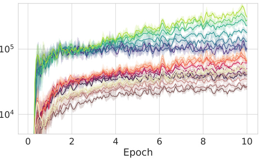
This figure shows the convergence rates of the largest NTK eigenvalue and sharpness with respect to width at multiple steps during training. It also shows the loss convergence rate and Hessian trace evolution. The key takeaway is that the sharpness exhibits width-independent behavior throughout training, unlike the NTK eigenvalue and loss, which show width dependence. This difference highlights the unique consistency of the sharpness across different model sizes.

This figure compares the training dynamics of sharpness (largest eigenvalue of the Hessian), loss, and learning rate across different model widths under two different parameterizations: µP and NTK. The µP parameterization shows consistent behavior across different widths (Super Consistency), with learning rate transfer. In contrast, the NTK parameterization shows significant discrepancies across widths, and no learning rate transfer. The results suggest a connection between Super Consistency of the loss landscape and learning rate transfer.

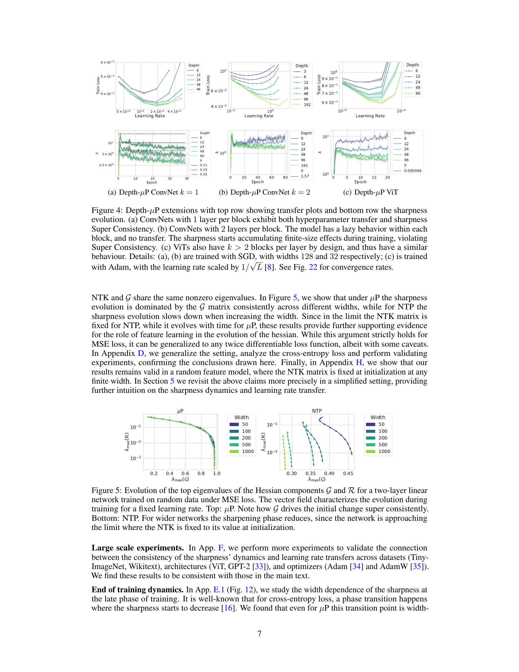
This figure compares the performance of three different network architectures (ConvNets with 1 layer per block, ConvNets with 2 layers per block, and ViTs) under the Depth-µP parameterization. The top row shows learning rate transfer plots, while the bottom row illustrates the sharpness evolution. The results demonstrate that networks with a single layer per block exhibit both hyperparameter transfer and sharpness Super Consistency (consistent sharpness dynamics across different model sizes). In contrast, networks with multiple layers per block (ConvNets with 2 layers per block and ViTs) show a lack of transfer and violate Super Consistency, indicating that sharpness dynamics are not consistent across different model sizes.

This figure shows the evolution of the top eigenvalues of the Hessian components G and R for a two-layer linear network trained on random data under MSE loss. The left panel shows the µP parameterization, where the sharpness evolution is largely dominated by the G matrix consistently across different widths. The right panel shows the NTP parameterization, where the sharpness evolution slows down when increasing the width. The results indicate that under µP, feature learning causes the progressive sharpening, while the lack of feature learning in NTP prevents the Hessian from adapting and its largest eigenvalue from reaching the convergence threshold.

This figure compares the training dynamics of sharpness and loss under two different parameterizations: µP and NTK. The top row shows that under µP scaling, the sharpness remains consistent across different model widths throughout training (a phenomenon the authors term ‘Super Consistency’), while the loss shows slight deviations at later stages. Importantly, the learning rate transfers effectively from smaller to larger models under µP. The bottom row demonstrates that under NTK parametrization, sharpness dynamics vary significantly across different widths, and the learning rate does not transfer. This highlights the relationship between Super Consistency and learning rate transfer.

This figure compares the training dynamics of sharpness and loss under µP and NTP parameterizations. The top row shows that under µP, sharpness remains consistent across different network widths (super consistency), while the loss eventually shows discrepancies due to finite-size effects. Learning rate transfer is observed under µP. The bottom row shows that under NTP, sharpness dynamics vary significantly across widths, and learning rate transfer does not occur. The experiment uses a two-layer convolutional neural network trained on CIFAR-10.

This figure compares the training dynamics of a two-layer convolutional neural network under two different parameterizations: µP and NTK. The top row shows the results under µP scaling, demonstrating that the sharpness (largest eigenvalue of the Hessian) remains consistent across different network widths throughout training (Super Consistency), while the training loss shows minor deviations with increasing width, and the optimal learning rate transfers from smaller to larger models. The bottom row illustrates the NTK parameterization, which shows significant differences in sharpness dynamics across different widths and a lack of learning rate transfer.

This figure compares the training dynamics of two-layer convolutional neural networks under two different parameterizations: µP and NTK. The top row shows results for µP, demonstrating that sharpness (a measure of landscape curvature) remains consistent across different network widths (‘Super Consistency’), while training loss shows some divergence with increasing width. Importantly, the learning rate transfers effectively between small and large models. In contrast, the bottom row shows results for NTK, where sharpness dynamics vary significantly with width, indicating inconsistent landscape behavior, and the learning rate does not transfer. This illustrates a key finding of the paper: learning rate transfer correlates with Super Consistency of the loss landscape.

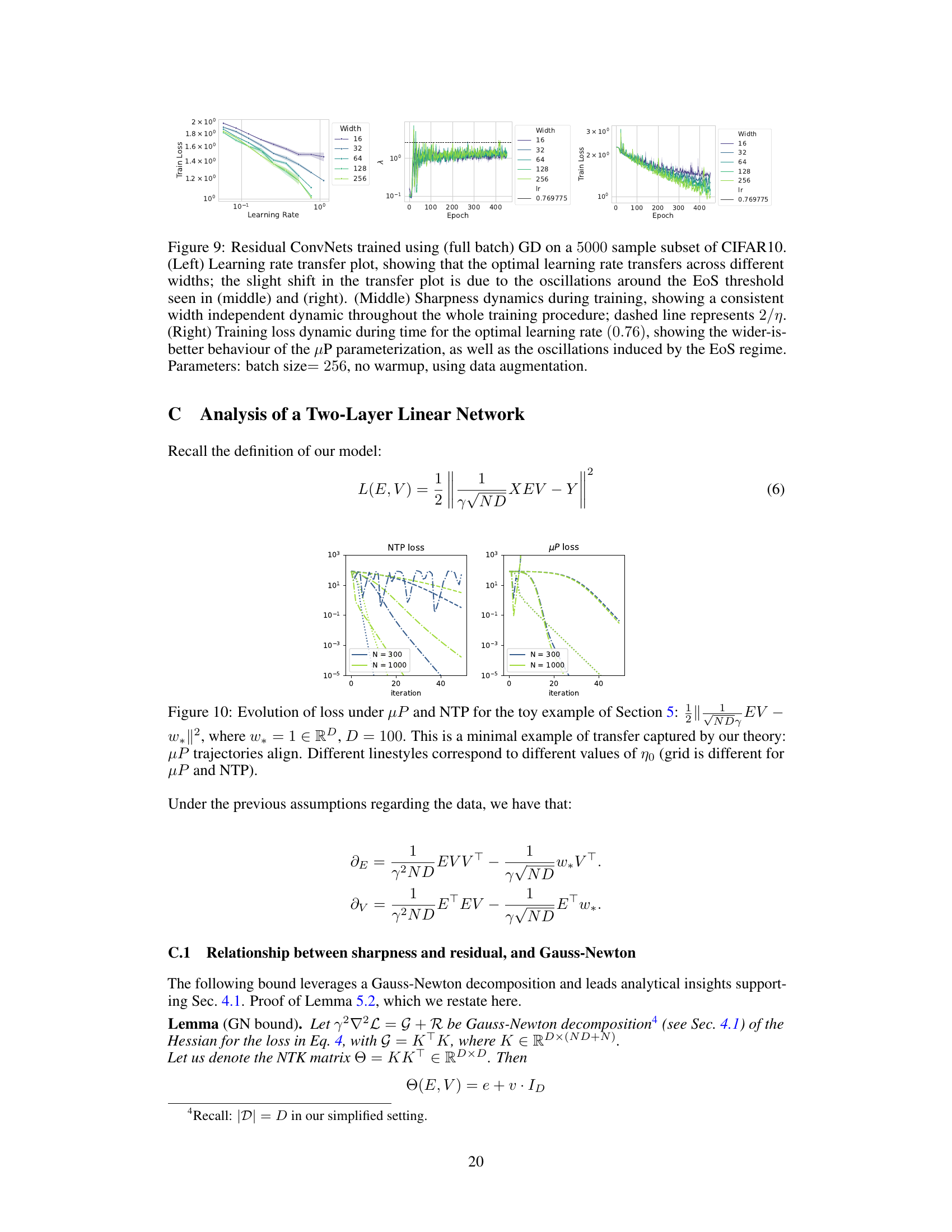
This figure shows the loss curves for a simple two-layer linear network with linear activation trained on a dataset with 100 dimensions. The network is trained under two different parameterizations: µP and NTP. The figure demonstrates the alignment of the loss curves across different learning rates under µP parameterization, illustrating the learning rate transfer phenomenon. Conversely, under NTP parameterization the curves do not align.

This figure visualizes the dynamics of the top Hessian eigenvalues and the top NTK eigenvalues during training of a 3-layer convolutional neural network. Panel (a) shows that the top Hessian eigenvalues progressively increase towards a threshold, and remain consistent across different network widths (super consistency). In contrast, panel (b) shows that the top NTK eigenvalues accumulate significant finite-size effects during training, with significant discrepancies across different widths. This difference highlights a key distinction between the µP and NTK parameterizations discussed in the paper.

This figure compares the training dynamics of sharpness and loss under µP (feature learning) and NTP (kernel regime) parameterizations. Under µP, the sharpness remains consistent across different network widths (Super Consistency), and the learning rate transfers from smaller to larger models. In contrast, under NTP, sharpness dynamics vary significantly with width, and learning rate transfer doesn’t occur. The experiment uses a two-layer convolutional network trained on CIFAR-10.
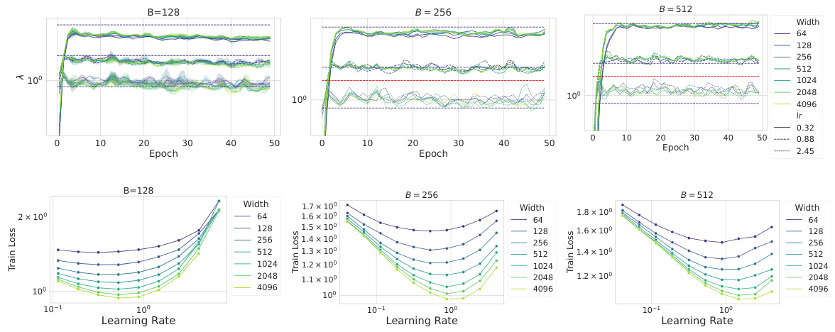
This figure demonstrates the key finding of the paper: Super Consistency. The top row shows that under the µP parameterization, the sharpness of the loss landscape (largest eigenvalue of the Hessian) remains largely consistent across different network widths throughout training. This is in contrast to the NTK parameterization (bottom row), where sharpness dynamics differ significantly across widths. The figure also highlights the relationship between Super Consistency and learning rate transfer; learning rate transfer is observed under µP but not NTK. The results are shown for a specific network architecture trained on CIFAR-10.

This figure compares the training dynamics of sharpness and loss under two different parameterizations: µP and NTK. The top row shows that under µP scaling, the sharpness remains consistent across different network widths throughout training (Super Consistency), while the loss shows some finite-size effects that accumulate over time. Importantly, the learning rate transfers successfully from smaller to larger models, indicating a consistent optimization landscape. In contrast, the bottom row shows the NTK parameterization, where the sharpness exhibits significant discrepancies across different widths and the learning rate does not transfer. This highlights the distinct behavior of the loss landscape under different scaling regimes and the crucial role of feature learning.

This figure compares the training dynamics of sharpness and loss under two different parameterizations: µP and NTK. The top row shows results for µP, demonstrating the consistent sharpness across different network widths (super consistency). The middle panel shows that the loss curves, while initially similar, diverge over time due to finite-size effects, violating super consistency. The right panel displays learning rate transfer from smaller to larger models under µP. The bottom row illustrates the NTK parameterization, revealing significant differences in sharpness dynamics and the absence of learning rate transfer. The experiment involves a two-layer convolutional network trained on CIFAR-10 with data augmentation.

This figure compares the training dynamics of a two-layer convolutional neural network under two different parameterizations: µP and NTK. The top row shows the results for µP, demonstrating that the sharpness (largest eigenvalue of the Hessian) remains consistent across different network widths throughout training, a phenomenon the authors term ‘Super Consistency.’ The training loss shows initial consistency but deviates over time due to finite-size effects. Importantly, the learning rate transfers effectively from smaller to larger networks. The bottom row illustrates the NTK parameterization, revealing significant discrepancies in sharpness dynamics across widths and a failure of learning rate transfer. This contrast highlights the key role of feature learning in achieving Super Consistency and learning rate transfer.

This figure compares the training dynamics of sharpness and loss under two different parameterizations (muP and NTK) across various network widths. The top row shows that under muP scaling, sharpness remains consistent across different widths (Super Consistency), while the loss eventually diverges. Learning rate transfers successfully from smaller to larger models under muP. The bottom row shows that under NTK scaling, sharpness dynamics differ significantly across widths and learning rate does not transfer. This highlights the importance of feature learning in achieving Super Consistency and learning rate transfer.

The figure compares the training dynamics of a two-layer convolutional neural network under two different parameterizations: µP (mu-P) and NTK (Neural Tangent Kernel). The top row shows results for µP. The leftmost plot demonstrates that the sharpness (largest eigenvalue of the Hessian) remains consistent across different network widths throughout training, a phenomenon the authors call ‘Super Consistency.’ The center plot shows that while the training loss is initially similar across widths, it diverges over time. The rightmost plot shows that the optimal learning rate transfers from small to large models under µP. The bottom row shows the analogous results for the NTK parameterization. In contrast to µP, the sharpness dynamics are vastly different at different scales, and the learning rate does not transfer.

This figure compares the training dynamics of two-layer convolutional neural networks under two different parameterizations: µP (muP) and Neural Tangent Kernel (NTK). The top row shows that under µP scaling, the sharpness (largest eigenvalue of the Hessian) remains consistent across different network widths throughout training, a phenomenon the authors term ‘Super Consistency.’ The training loss shows some initial similarity but diverges over time, and the learning rate transfers successfully from smaller to larger models. The bottom row demonstrates that under NTK scaling, the sharpness dynamics differ significantly across widths and the learning rate does not transfer.
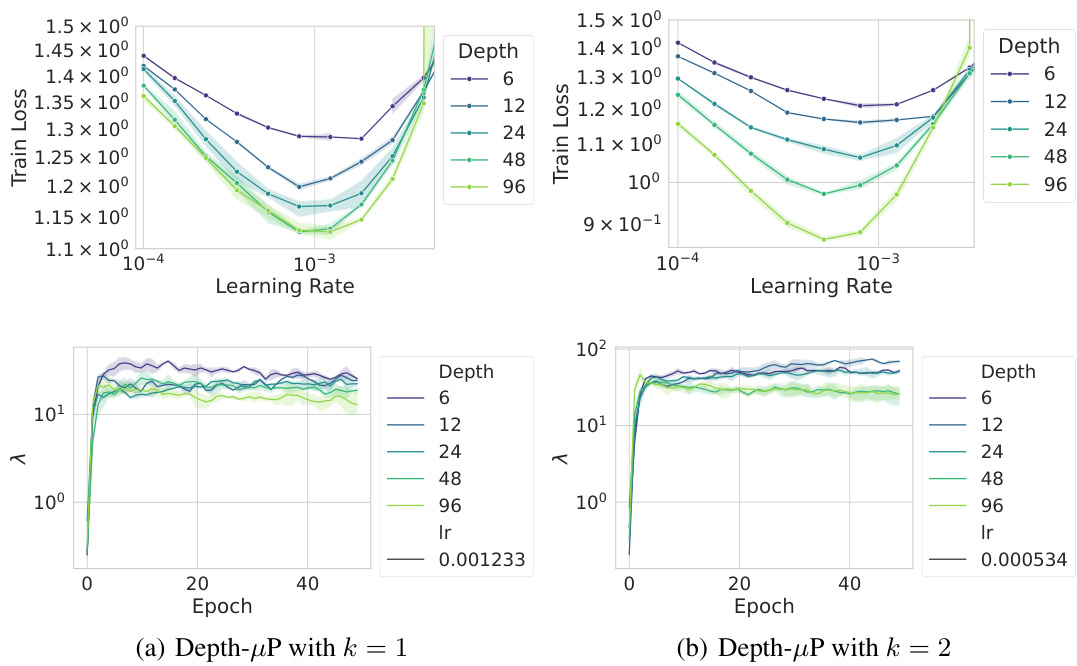
This figure shows the results of experiments using Depth-µP scaling with different numbers of layers per residual block. The top row displays learning rate transfer plots and the bottom row shows sharpness evolution across different model widths and depths. Part (a) demonstrates both hyperparameter transfer and Super Consistency with one layer per block. In contrast, (b) and (c), which employ two or more layers per block, respectively, do not exhibit transfer, and their sharpness shows increasing deviations with width and depth, indicating a lack of Super Consistency. This suggests that the Super Consistency property of the loss landscape is crucial for learning rate transfer across different model sizes. The specific architectures include convolutional networks and Vision Transformers.
This figure compares the training dynamics of sharpness and loss under two different parameterizations: µP and NTK. µP exhibits ‘Super Consistency,’ meaning the sharpness remains consistent across different network widths throughout training. The learning rate also transfers between models of different sizes. In contrast, the NTK parametrization shows significantly different sharpness dynamics at different scales, and the learning rate does not transfer.
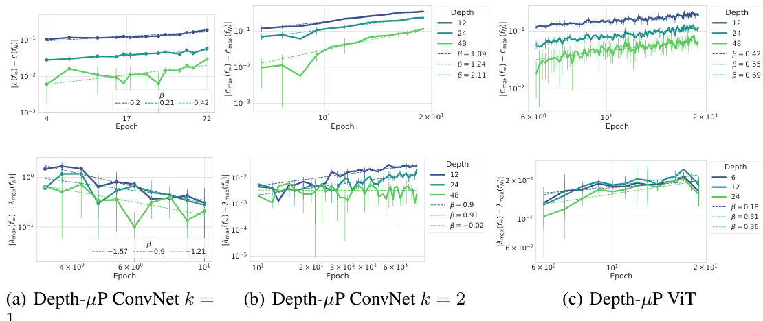
This figure shows the convergence rates of losses and sharpnesses over time for three different network architectures: Depth-µP ConvNet with k=1, Depth-µP ConvNet with k=2, and Depth-µP ViT. Each plot shows the convergence rate (fitted power law y=atβ) of the loss and sharpness (largest eigenvalue of the preconditioned Hessian) for various network depths. The results illustrate differences in how the consistency of the sharpness and loss varies depending on the architecture and scaling regime.
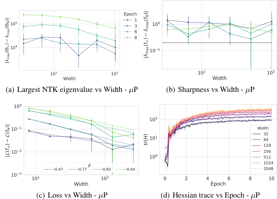
This figure analyzes the convergence rate of different properties of the loss landscape (largest NTK eigenvalue, sharpness, loss, and Hessian trace) with respect to the network width. It shows that while the sharpness remains consistent across different widths, other quantities like the largest NTK eigenvalue and the loss accumulate finite-size effects as width increases. The Hessian trace also exhibits width dependence initially but converges to a width-independent value.
The figure shows the training dynamics of sharpness and loss for both µP and NTK parameterizations across various model widths. Under µP, sharpness remains consistent regardless of width, exhibiting a phenomenon called ‘Super Consistency’, while the loss shows some deviation. Learning rate transfer is also observed under µP, but not under NTK, where sharpness displays significant variation across different widths. This suggests a link between Super Consistency and learning rate transfer.

This figure shows the training dynamics of the top eigenvalues of the Hessian and Neural Tangent Kernel (NTK) matrices under µP parametrization. The top row (a) shows that the largest Hessian eigenvalues exhibit Super Consistency, converging to a width-independent threshold, while the smaller eigenvalues show finite-size effects. The bottom row (b) shows that the top NTK eigenvalues show significant finite-size effects during training, in contrast to the Hessian eigenvalues. This difference highlights the impact of feature learning on the landscape’s properties.

This figure compares the training dynamics of a two-layer convolutional neural network under two different parameterizations: µP (mu-P) and NTK (Neural Tangent Kernel). The top row shows results for the µP parameterization. The left plot demonstrates that the sharpness (largest eigenvalue of the Hessian) remains consistent across different network widths throughout training, a phenomenon the authors term ‘Super Consistency.’ The center plot shows that while training loss is initially similar, finite-size effects accumulate over time, violating Super Consistency. The right plot shows that the optimal learning rate transfers from small to large models, further supporting the idea of Super Consistent loss landscapes. The bottom row shows results for the NTK parameterization. In contrast to µP, the sharpness dynamics exhibit significant discrepancies across different widths, and the learning rate does not transfer. This suggests that Super Consistency is linked to learning rate transfer.

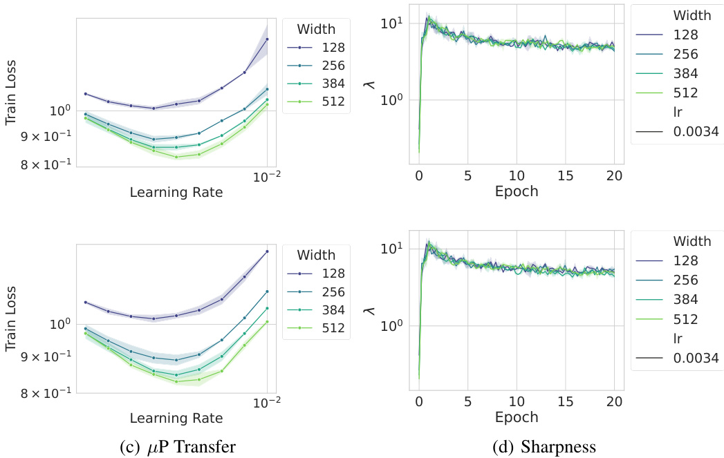
This figure shows the results of training convolutional neural networks on CIFAR-10 using two different parameterizations: µP (top) and Depth-µP (bottom). Both parameterizations aim to achieve learning rate transfer, meaning the optimal learning rate remains consistent across different model sizes (widths for µP, depths for Depth-µP). The left panels (a and c) illustrate this learning rate transfer, with each line representing a different model size. The right panels (b and d) demonstrate Super Consistency of the landscape, a property the authors define where the alignment between the gradient and the Hessian’s largest eigenvalues remains consistent throughout the training process. The dashed lines in (b and d) represent the Edge of Stability (EoS) threshold.

This figure compares the training dynamics of sharpness (largest eigenvalue of the Hessian), training loss, and learning rate for two different model scaling methods: µP and NTK. Under µP scaling, the sharpness remains consistent across different model widths, showing a phenomenon the authors call ‘Super Consistency.’ The training loss shows some consistency early on but diverges over time, while the learning rate transfers effectively between small and large models. In contrast, under NTK scaling, the sharpness dynamics differ significantly across widths, and learning rate transfer does not occur. The experiment uses a two-layer convolutional network trained on the CIFAR-10 dataset.
Full paper#

