↗ OpenReview ↗ NeurIPS Homepage ↗ Chat
TL;DR#
Many existing dynamic graph learning models struggle with out-of-distribution (OOD) generalization, especially due to changes in temporal environments. These models often fail to accurately infer and utilize environmental information, leading to poor performance on unseen data. This paper tackles this challenge by focusing on both environment inference and utilization.
The proposed model, Environment-prompted Dynamic Graph Learning (EpoD), uses a novel self-prompted learning mechanism to infer unseen environment factors. Instead of relying on predefined environment scales, it learns environment representations directly from the data. EpoD also incorporates a structural causal model with dynamic subgraphs, which act as mediating variables. These subgraphs effectively capture the impact of environment shifts on data correlations. Extensive experiments show that EpoD outperforms existing methods in terms of both accuracy and interpretability, demonstrating its effectiveness in handling temporal OOD generalization.
Key Takeaways#
Why does it matter?#
This paper is crucial for researchers working on dynamic graph learning, particularly those focusing on out-of-distribution (OOD) generalization. It addresses the critical issue of temporal OOD, offering a novel approach to improve model robustness and interpretability. The proposed method, along with the theoretical analysis and extensive experiments, provides valuable insights and sets a new benchmark for future research in this area. The interpretability aspect of the model is also valuable, which can open new avenues for further research and applications.
Visual Insights#

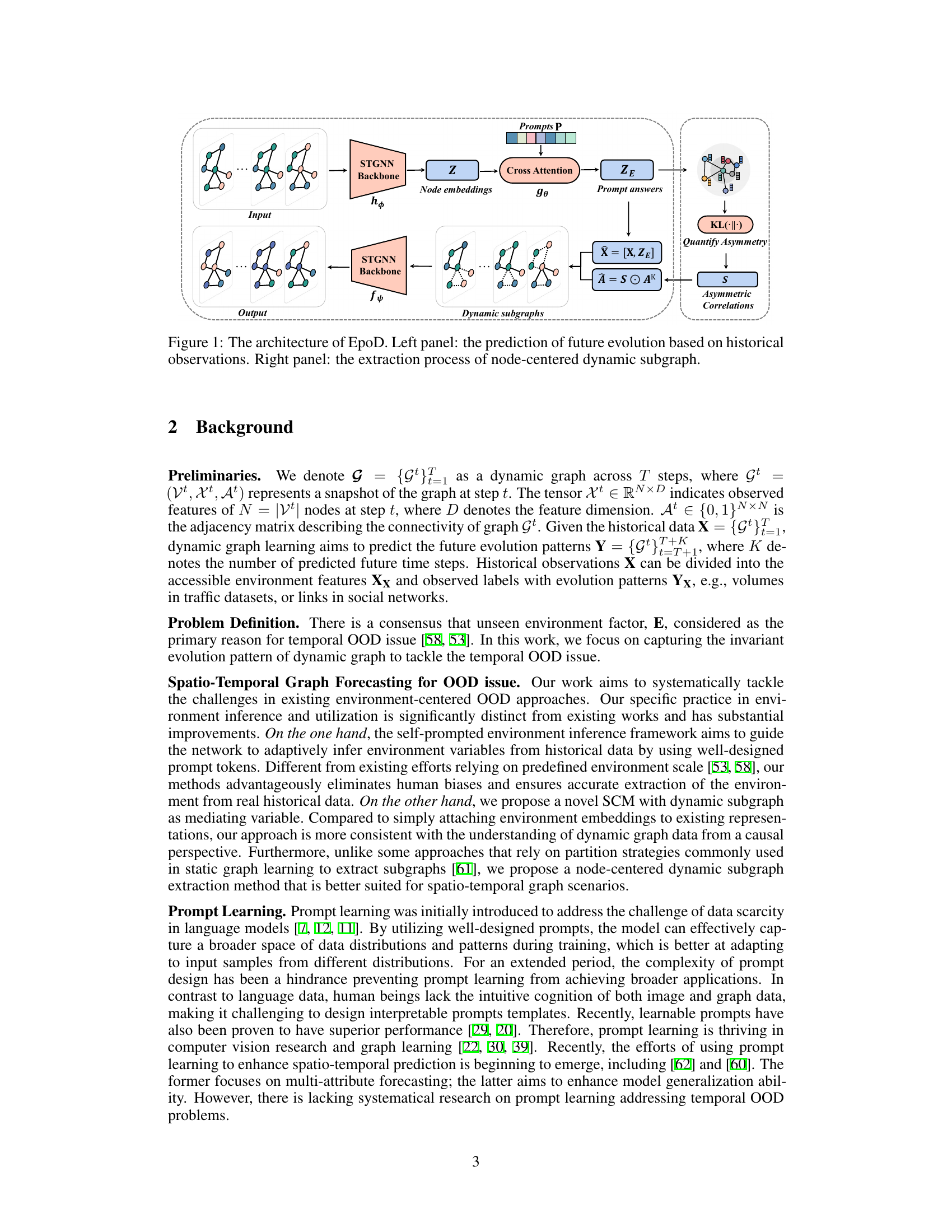
This figure illustrates the architecture of the proposed Environment-prompted Dynamic Graph Learning (EpoD) model. The left panel shows the prediction process, where historical observations are input to a spatio-temporal graph neural network (STGNN) backbone to obtain node embeddings. These embeddings are then processed by a cross-attention mechanism with prompts to generate prompt answers which help infer unseen environment variables. These variables are incorporated into the STGNN backbone along with the original input to predict future evolution. The right panel shows how node-centered dynamic subgraphs are extracted. The asymmetry between node correlations is quantified using Kullback-Leibler divergence and then used to create dynamic subgraphs. These subgraphs effectively capture distribution shifts due to changes in the environment.

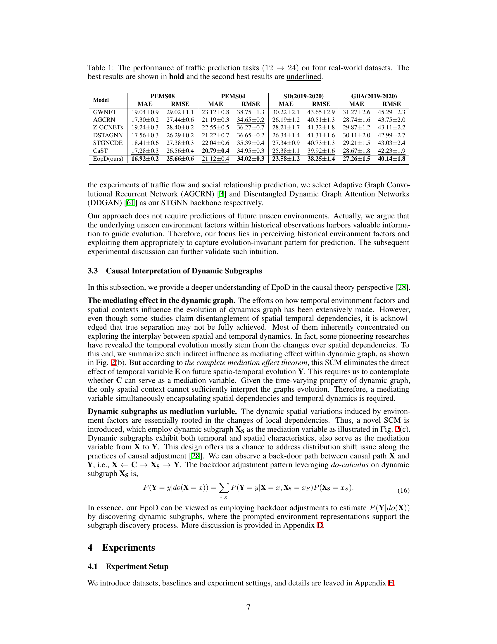
This table presents the performance comparison of several traffic flow prediction models on four real-world datasets (PEMS08, PEMS04, SD, GBA). The models are evaluated using two metrics: Mean Absolute Error (MAE) and Root Mean Squared Error (RMSE). Lower values of MAE and RMSE indicate better performance. The results show that the proposed model, EpoD, achieves the best performance on three out of four datasets, demonstrating its effectiveness and superiority over other state-of-the-art models.
In-depth insights#
Env-Prompted DGL#
Env-Prompted Dynamic Graph Learning (DGL) represents a novel approach to enhance the generalization capabilities of DGL models, particularly in handling out-of-distribution (OOD) scenarios. The core idea is to incorporate environmental factors into the learning process, enabling the model to better adapt to unseen environmental conditions. This is achieved through a two-pronged strategy: 1) inferring underlying environment factors using a self-prompted learning mechanism and 2) leveraging a structural causal model with dynamic subgraphs as mediating variables to capture the influence of environment shifts on the data distribution. The self-prompted learning mechanism avoids predefining environment scales, allowing for more robust and accurate inference of unseen environments. By incorporating inferred environmental variables into a causal model with dynamic subgraphs, the model gains enhanced adaptability to environmental changes, leading to improved OOD generalization. This approach offers a significant advancement by systematically addressing the issues of environment inference and utilization. The framework’s effectiveness is demonstrated across various real-world dynamic graph datasets, showcasing superior performance against baseline methods and strong interpretability.
Self-Prompted Learning#
Self-prompted learning represents a significant advancement in tackling the challenge of unseen environments in dynamic graph learning. By sidestepping the limitations of predefined environment scales, this approach leverages the power of prompt learning to infer environment representations directly from historical data. This autonomous learning mechanism is particularly valuable when explicit environment labels are absent. The core idea is to guide the model to extract informative environment variables by using learnable prompt tokens, thus eliminating the need for human intervention in defining environment characteristics. The interaction between prompts and the model’s learned embeddings is crucial, allowing for a compact and nuanced representation of the environment’s impact on the graph’s evolution. This approach’s strength lies in its ability to adapt to a wide range of environments without restrictive predefined scales, enhancing the model’s generalizability and robustness. However, the success heavily hinges on designing effective prompt structures and an interactive squeezing mechanism, which requires a careful consideration of spatio-temporal relationships within the dynamic graph. Further exploration could investigate optimal prompt design strategies and the sensitivity of performance to different prompt architectures.
Dynamic Subgraph#
The concept of ‘Dynamic Subgraph’ in the context of dynamic graph learning is crucial for capturing the evolving relationships between nodes over time. Static subgraph methods are insufficient because they fail to adapt to the changing dependencies induced by shifting environments or other dynamic factors. A dynamic subgraph approach acknowledges that the relationships between nodes are not static but change over time and these changes are often asymmetric. Node-centered subgraphs are particularly beneficial as they reflect how each node’s connectivity evolves uniquely, influenced by its changing interactions within the system. The key is to extract subgraphs that meaningfully reflect these changing relationships, such as using node-centered approaches or other methods that capture asymmetric dependencies. By incorporating the learned dynamic subgraphs into a causal model, one can better account for the influence of environment factors, improving the model’s generalization ability and providing a more interpretable framework for understanding spatio-temporal dynamics. The effective capture of asymmetric correlations between nodes through dynamic subgraphs is key to understanding and modeling the evolution of dynamic graphs, thus addressing the out-of-distribution (OOD) generalization challenge.
Causal Interpretation#
A causal interpretation of a model’s behavior is crucial for understanding its decision-making process and ensuring reliable predictions, especially in complex domains. By framing the problem through a causal lens, we can disentangle direct and indirect effects of variables, revealing underlying mechanisms. This approach not only improves the model’s transparency and interpretability but also enhances its robustness to distribution shifts and out-of-distribution generalization, as causal relationships are often more stable than purely statistical correlations. In the context of dynamic systems, a causal approach facilitates the identification of mediating variables that convey the influence of environment factors on system evolution, which improves model’s ability to adapt to changing conditions. This is particularly important in dynamic graph learning where environmental changes induce alterations in both node features and relationships. A causal interpretation helps to understand how these changes propagate and affect the overall prediction accuracy. By understanding the underlying causal structure, we can design more effective interventions to influence the system’s behavior, making it more controllable and predictable. Furthermore, a causal perspective allows us to identify and account for confounding factors and spurious correlations, ultimately leading to more accurate and reliable models.
OOD Generalization#
Out-of-distribution (OOD) generalization, a critical aspect of robust machine learning, is profoundly challenged in dynamic graph learning. Temporal environmental changes are a primary source of distribution shifts, impacting model performance on unseen data. Existing methods often struggle with environment inference and effective utilization, sometimes relying on pre-defined environment representations that may be unrealistic. A promising direction involves inferring the underlying environment factors from data and leveraging this information to enhance model generalization. Prompt learning emerges as a powerful tool to infer unseen environment representations directly from data, bypassing pre-defined codebooks. Causal modeling, specifically incorporating dynamic subgraphs as mediating variables, offers a more robust and interpretable way to utilize inferred environmental factors, capturing how changes in environments affect spatio-temporal dependencies within the graph. This approach emphasizes capturing the invariant structure of the graph evolution across various environmental conditions, rather than simply treating environment variables as additional features. Thus, future research should focus on more sophisticated prompt learning techniques and causal modeling frameworks that address the complex challenges of OOD generalization in dynamic graph learning.
More visual insights#
More on figures

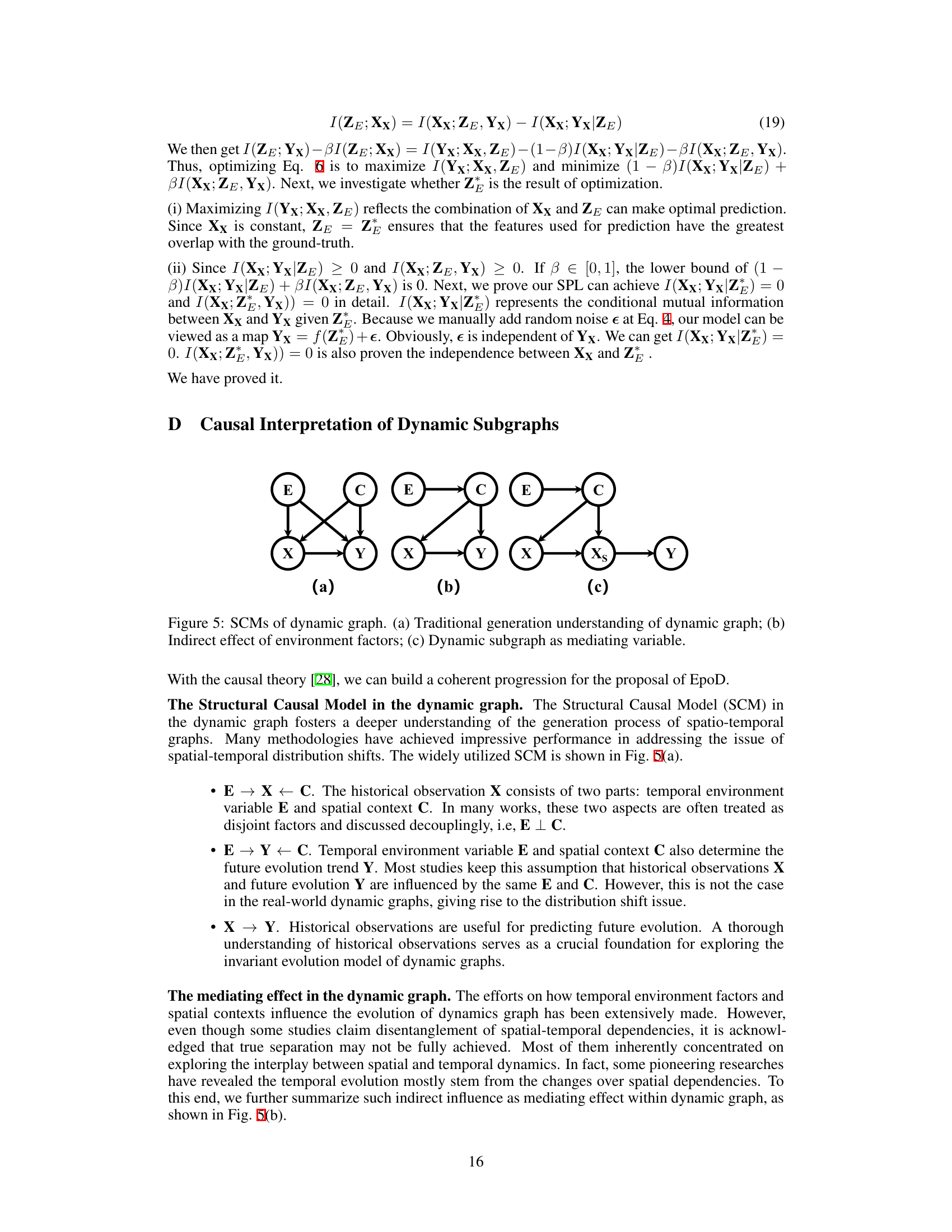
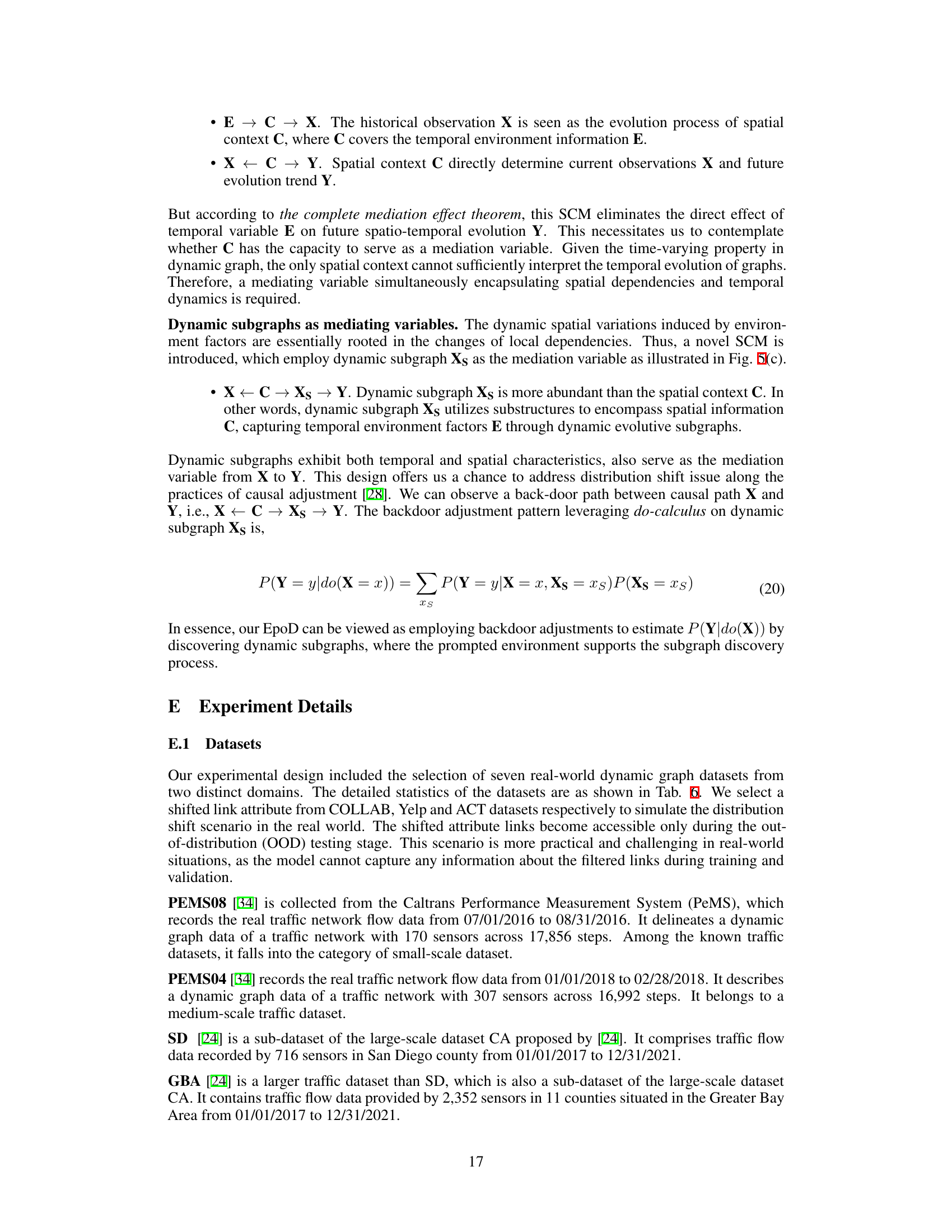
This figure illustrates three structural causal models (SCMs) depicting the influence of environment factors and spatial contexts on the evolution of dynamic graphs. (a) shows a traditional SCM where environment (E) and context (C) directly influence both historical observations (X) and future evolution (Y). (b) shows an indirect effect, where environment factors indirectly influence Y through C and X. (c) introduces a novel SCM using dynamic subgraphs (Xs) as a mediating variable. This model acknowledges the impact of environment variables on the correlations between nodes within the dynamic graphs and introduces dynamic subgraphs to capture the evolving structural associations.

This figure shows the distribution difference between masked feature XB and prompted environment feature ZE in two scenarios: sharp temporal distribution shift and temporal distribution shift with slight signals. The left panel (a) shows that the prompted environment variables can cover more than half of the shifted features even in the case of a sharp shift. The right panel (b) demonstrates that the prompted environment variables effectively capture even slight early signals, indicating their ability to handle OOD issues. The light blue shading represents the standard deviation.

This figure compares three different approaches for designing learnable prompts: SingleP (a single globally shared prompt), EpoD (the proposed method with node-wise learnable prompts), and PrivateP (node-private learnable prompts). It shows the time consumption (in seconds per epoch) and the performance (MAE) for each approach across three different datasets (PEMS08, PEMS07, PEMS04). The results demonstrate that EpoD achieves a balance between computational efficiency and prediction accuracy, outperforming SingleP while maintaining comparable efficiency to PrivateP.

This figure shows three structural causal models (SCMs) illustrating different understandings of dynamic graphs. (a) shows a traditional SCM where the environment (E) and context (C) directly influence both historical observations (X) and future outcomes (Y). (b) illustrates an indirect effect, where E influences Y through C. (c) introduces a mediating variable, the dynamic subgraph (Xs), which captures the influence of E and C on Y, thereby improving adaptability to environmental changes.

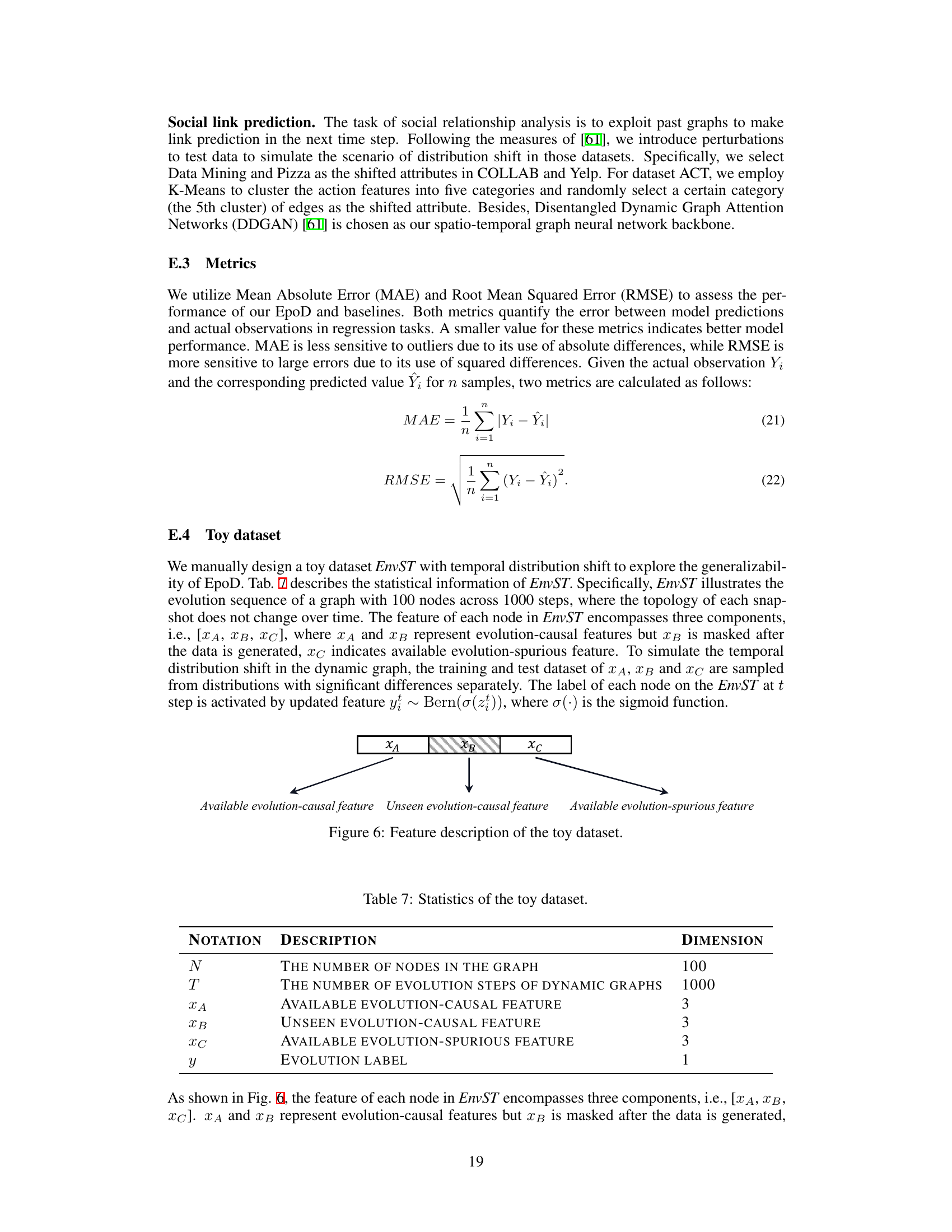
The figure shows the composition of features in the toy dataset EnvST. It consists of three components: XA (available evolution-causal feature), XB (unseen evolution-causal feature, masked after data generation), and XC (available evolution-spurious feature). The figure illustrates how these features are combined and their impact on the evolution label (y).
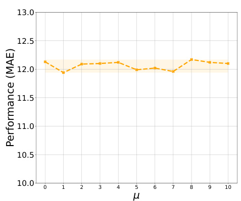
This figure shows the results of an experiment on a toy dataset (EnvST) designed to test the model’s ability to handle spurious correlations. The x-axis represents the mean (μ) of the spurious information, and the y-axis represents the model’s performance (MAE). The shaded area represents the acceptable error bounds. The plot demonstrates that the model’s performance remains consistently within these bounds despite varying levels of spurious information, suggesting its robustness to such noise.

The figure shows the sensitivity analysis of the hyperparameter β on four real-world datasets: PEMS08, PEMS04, SD, and Yelp. The x-axis represents the value of β, and the y-axis represents the performance (MAE) of the model. The shaded area represents the standard deviation of the performance. The results show that the performance of the model is not very sensitive to the value of β, but the best performance is achieved when β is around 0.2.
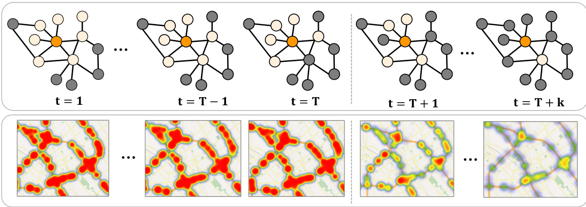
This figure shows the interpretability of dynamic subgraphs in real-world scenarios, specifically focusing on the impact of the COVID-19 pandemic on traffic flow. The top panel visualizes the dynamic subgraphs extracted by the proposed EpoD model at different time steps, illustrating how the communication among nodes (representing sensors in a traffic network) changes over time, particularly around three key nodes (shown in blue). The bottom panel displays the ground-truth of traffic flow, showing a similar pattern in suppressed communication during the pandemic’s distribution shift. This demonstrates the model’s ability to capture the changes in spatial dependencies that reflect real-world events.
More on tables

This table presents the Area Under the Curve (AUC) scores, a metric for evaluating the performance of link prediction models on social relationship datasets. It compares the performance of several models (DySAT, IRM, VREx, GroupDRO, DIDA, EAGLE, and the proposed EpoD) across three datasets (Collab, Yelp, and ACT). Higher AUC scores indicate better performance. The best and second-best results for each dataset are highlighted in bold and underlined, respectively.

This table presents the ablation study results comparing three versions of the EpoD model: EpoD-NoSub (without dynamic subgraphs), EpoD-PartitionSub (with partition-based subgraph extraction), and EpoD (the proposed model with node-centered dynamic subgraphs). The results, in terms of MAE (Mean Absolute Error) for traffic flow prediction datasets PEMS08 and PEMS04, and AUC (Area Under the Curve) for the social network dataset Yelp, demonstrate the impact of incorporating dynamic subgraphs on model performance and the superiority of the proposed node-centered approach.
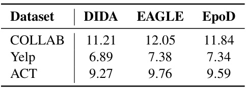
This table presents the efficiency analysis of the proposed EpoD model in terms of seconds per epoch (s/epoch) for different datasets. It compares EpoD’s efficiency against two other models, DIDA and EAGLE, across three datasets: COLLAB, Yelp, and ACT. Lower numbers indicate better efficiency.

This table presents the Mean Absolute Error (MAE) and Root Mean Squared Error (RMSE) for traffic flow prediction tasks on four real-world datasets: PEMS08, PEMS04, SD(2019-2020), and GBA(2019-2020). The table compares the performance of the proposed EpoD model against several baseline models (GWNET, AGCRN, Z-GCNETS, DSTAGNN, STGNCDE, CaST). The best and second-best results for each dataset and metric are highlighted in bold and underlined, respectively. The results demonstrate the superior performance of EpoD for long-sequence traffic flow prediction.

This table presents a comparison of the Mean Absolute Error (MAE) and Root Mean Squared Error (RMSE) for traffic flow prediction across four real-world datasets (PEMS08, PEMS04, SD, and GBA). The models compared include GWNET, AGCRN, Z-GCNETS, DSTAGNN, STGNCDE, CaST, and the proposed EpoD model. The results are shown for a 12-step prediction task (predicting the next 24 time steps given the previous 12). The best performing model for each metric on each dataset is highlighted in bold, while the second-best is underlined.

This table presents the Mean Absolute Error (MAE) and Root Mean Squared Error (RMSE) for traffic flow prediction on four real-world datasets using different models. The task is to predict the next 24 time steps given the previous 12 time steps. The models compared include GWNET, AGCRN, Z-GCNETs, DSTAGNN, STGNCDE, CaST, and the proposed EpoD model. The best performing model for each metric on each dataset is highlighted in bold, with the second best underlined. This allows for a comparison of model performance across different datasets and metrics, showcasing the effectiveness of the proposed model.

This table shows the Mean Absolute Error (MAE) achieved by the EpoD model on the PEMS08 dataset for different values of the hyperparameter L used in Equation 12. The hyperparameter L controls the size of the node-centered dynamic subgraph used in the model, with a larger value indicating a larger subgraph. The table shows the MAE for values of L ranging from 1 to 10, illustrating how the model’s performance changes with varying subgraph sizes. This analysis helps to determine the optimal value of L for balancing performance and computational cost.

This table presents the Mean Absolute Error (MAE) and Root Mean Squared Error (RMSE) for traffic flow prediction tasks on four real-world datasets: PEMS08, PEMS04, SD(2019-2020), and GBA(2019-2020). It compares the performance of the proposed EpoD model against several baseline models, namely GWNET, AGCRN, Z-GCNETS, DSTAGNN, STGNCDE, and CaST. The results show MAE and RMSE values for each model on each dataset, with the best performing model for each dataset highlighted in bold and the second-best underlined. This allows for a direct comparison of the EpoD model’s performance against existing state-of-the-art methods on a variety of traffic flow datasets.
Full paper#
