↗ OpenReview ↗ NeurIPS Homepage ↗ Chat
TL;DR#
Transformer-based models have shown promise in time series forecasting, but they struggle with limited semantic information in individual time points and entangled temporal variations across different scales. These challenges hinder their ability to accurately capture the complex patterns inherent in real-world time series data. Existing methods often rely on simple pair-wise interactions or predefined structures, failing to fully exploit the richness of the data.
Ada-MSHyper addresses these issues by employing an adaptive hypergraph learning module to capture group-wise interactions more effectively. A multi-scale interaction module further refines pattern recognition by considering interactions across different scales. This innovative approach, combined with a novel node and hyperedge constraint mechanism, leads to improved accuracy and state-of-the-art results on multiple benchmark datasets, demonstrating the potential of Ada-MSHyper for diverse time series forecasting applications. The method significantly outperforms other state-of-the-art methods across various time series lengths, demonstrating its robustness and generalizability.
Key Takeaways#
Why does it matter?#
This paper is important because it addresses critical limitations of existing transformer-based time series forecasting methods. By introducing adaptive hypergraph learning and multi-scale interaction modules, it significantly improves forecasting accuracy across various time series lengths and complexities. This work opens new avenues for research in hypergraph neural networks and their applications to time series forecasting, impacting researchers in machine learning, data mining, and various application domains that deal with time-dependent data. The improvements in accuracy are substantial across many benchmarks, and make the proposed method a strong contender for real-world applications.
Visual Insights#
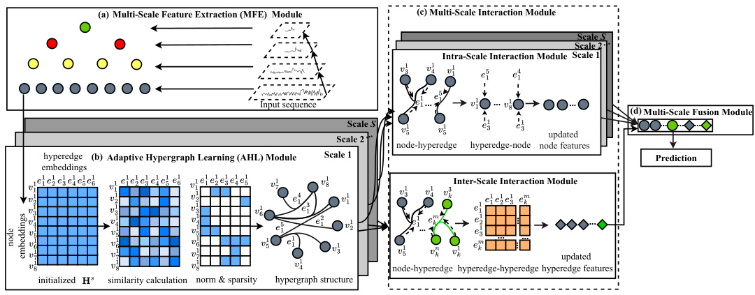
The figure shows the overall framework of the Ada-MSHyper model. It consists of four main modules: (a) Multi-Scale Feature Extraction (MFE) Module, which extracts feature representations at different scales; (b) Adaptive Hypergraph Learning (AHL) Module, which automatically generates incidence matrices to model implicit group-wise node interactions at different scales; (c) Multi-Scale Interaction Module, which performs both intra-scale and inter-scale interactions using hypergraph convolution attention; and (d) Multi-Scale Fusion Module, which combines multi-scale information for prediction. The figure illustrates the flow of information through these modules and highlights the key components of the Ada-MSHyper model.

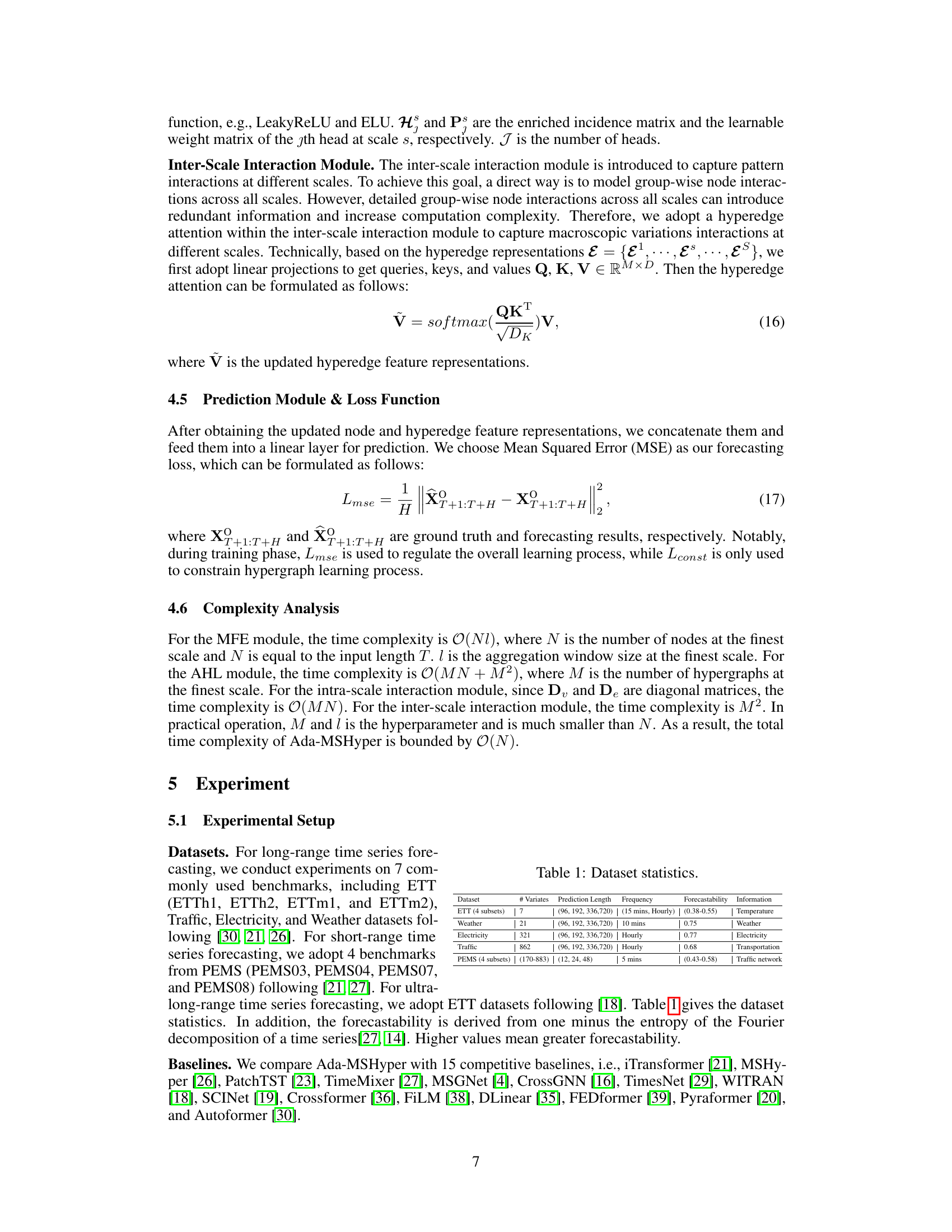
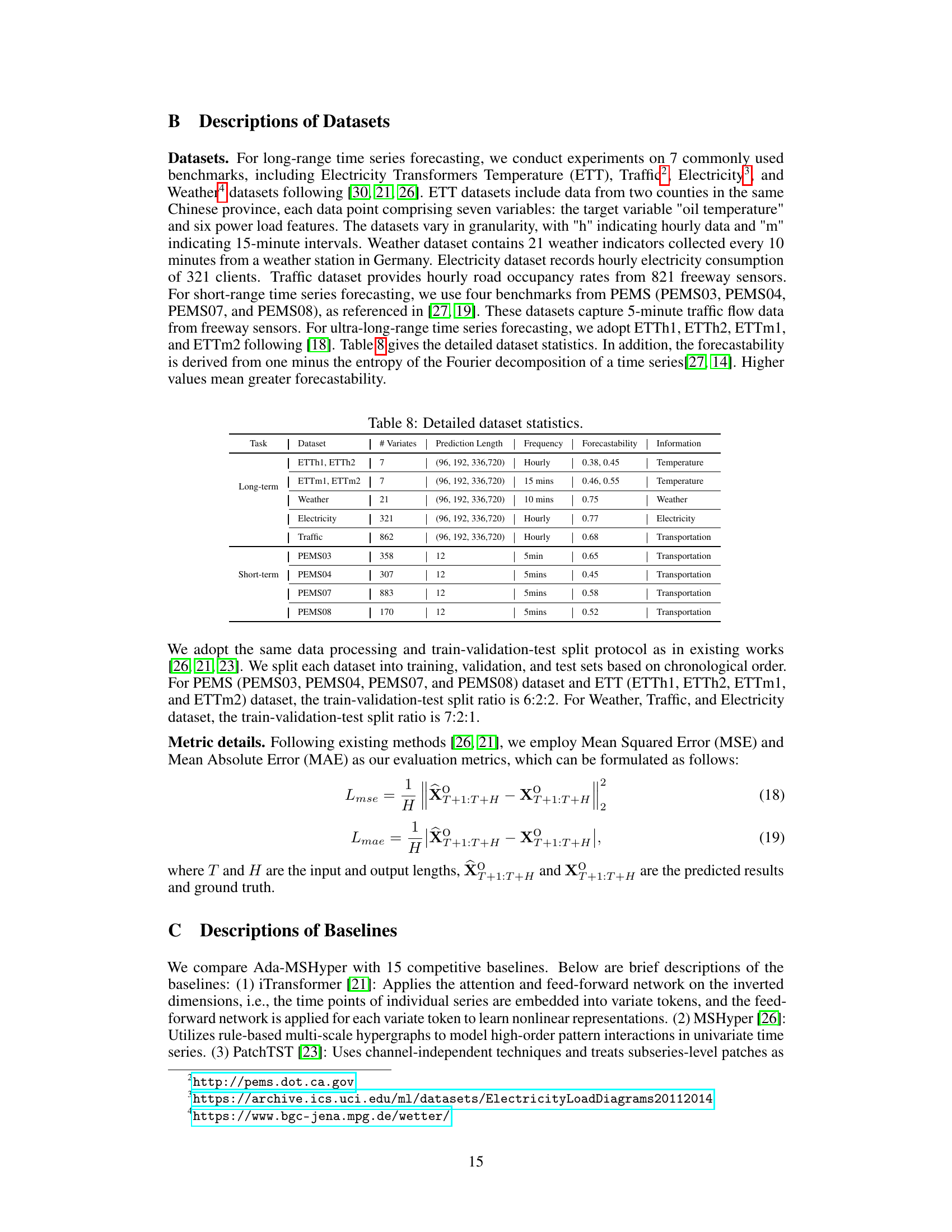
This table provides a summary of the characteristics of the eleven datasets used in the paper’s experiments. For each dataset, it shows the number of variables (# Variates), the prediction lengths considered, the frequency of data collection, a measure of the dataset’s predictability (Forecastability), and a description of the information contained within.
In-depth insights#
Adaptive Hypergraph#
The concept of “Adaptive Hypergraph” in the context of a time series forecasting model suggests a dynamic and data-driven approach to capturing complex relationships within the data. Unlike static hypergraphs with predefined structures, an adaptive hypergraph learns and adjusts its connections based on the inherent patterns and characteristics of the time series. This adaptability is crucial for effectively modeling the intricate and often non-linear relationships present in real-world time series data which may exhibit diverse temporal patterns at multiple scales. The model likely uses a learning algorithm to determine the optimal hyperedge connections, potentially incorporating node similarity measures or other criteria to define the strength of relationships within the graph. This dynamic aspect allows the model to automatically adapt to various types of time series, such as long-range, short-range, and ultra-long-range, and to capture both abundant and implicit group-wise interactions among data points. The adaptive nature allows it to handle diverse temporal variations (rising, falling, fluctuating), which traditional methods often struggle with by disentangling and modeling them effectively. Furthermore, the adaptive hypergraph likely enhances the model’s ability to handle noise interference while preserving the inherent semantic information within the time series for better forecasting accuracy.
Multi-Scale Modeling#
Multi-scale modeling in time series forecasting aims to capture temporal patterns across various granularities. Successfully addressing this requires methods capable of handling both short-term, high-frequency fluctuations and long-term, low-frequency trends. Simple models often fail to capture this complexity. Advanced techniques, such as those employing wavelets, or multi-resolution analysis, decompose the time series into different frequency components. This allows for separate modeling of different scales, improving accuracy and interpretability. However, the choice of decomposition method and the way the multiple scales are integrated are critical. A poorly chosen approach might lose important information or introduce artifacts. Effective multi-scale modeling demands careful consideration of data characteristics, computational cost, and the specific forecasting task. The ideal method should seamlessly combine information from multiple scales, enhancing the overall forecasting performance. Furthermore, the ability to adaptively adjust to varying scales within the time series, rather than relying on fixed-scale decompositions, is key to robust performance on complex, real-world data.
Temporal Variations#
Analyzing temporal variations in time series data is crucial for accurate forecasting. Variations represent the inherent dynamic patterns within data, deviating from simple trends or seasonality. Understanding these variations is key to building effective forecasting models. Multiple types of variations may exist simultaneously, like rising, falling, and fluctuating patterns, which can be intertwined and difficult to disentangle. Methods for addressing these complexities include series decomposition, separating trends from seasonality and noise, and multi-periodicity analysis, identifying recurring patterns across various timescales. Advanced techniques such as adaptive hypergraph modeling provide a novel approach, capturing complex interactions and implicit relationships between different temporal variations. Effective modeling of temporal variations ultimately leads to more accurate and robust forecasting, enhancing the predictive power of time series models in various applications.
Future Research#
The paper’s “Future Research” section suggests several promising avenues. Extending the framework to 2D spectrogram data could significantly improve the model’s ability to capture intricate temporal patterns in time-frequency domains. This approach would allow the model to leverage richer feature representations. Furthermore, developing a disentangled multi-scale feature extraction module is proposed to reduce redundancy and improve the model’s efficiency. This suggests that the authors are aware of potential limitations in their current feature extraction, and aim to improve upon this aspect. Finally, they highlight the need for more extensive datasets to better evaluate the model’s generalization capabilities, suggesting an awareness of current data limitations and a desire for more robust evaluation. These future directions show a commitment to refining existing methodology and addressing identified shortcomings, strengthening the overall work’s potential impact.
Limitations Addressed#
The research paper addresses the limitations of existing transformer-based methods in multi-scale time series forecasting. Semantic information sparsity, a common issue in time series where individual data points lack rich semantic context, is tackled by employing an adaptive hypergraph learning module to capture group-wise interactions. This moves beyond pairwise attention, allowing for the incorporation of more contextual information. The second limitation tackled is temporal variations entanglement, where inherent variations (rising, falling, fluctuating) within time series patterns overlap and hinder accurate forecasting. The paper introduces a multi-scale interaction module and a novel node and hyperedge constraint mechanism to untangle these variations at different scales, improving the model’s ability to differentiate temporal patterns. Adaptive hypergraph learning allows the model to discover intricate relationships between data points rather than relying on pre-defined structures, leading to more accurate and robust predictions. The combination of these approaches significantly improves forecasting performance over existing methods.
More visual insights#
More on figures

This figure shows the overall framework of the proposed Ada-MSHyper model for time series forecasting. It consists of four main modules: 1) Multi-Scale Feature Extraction (MFE) module which extracts feature representations at different scales. 2) Adaptive Hypergraph Learning (AHL) module that automatically generates incidence matrices to model implicit group-wise node interactions at different scales. 3) Multi-Scale Interaction Module which performs intra-scale and inter-scale interactions. 4) Prediction Module that generates the final prediction. The figure also highlights the node and hyperedge constraint mechanism (NHC) that is used to cluster nodes with similar semantic information and differentiate temporal variations within each scale.

This figure shows the overall framework of the Ada-MSHyper model, which consists of four main modules: (a) Multi-Scale Feature Extraction (MFE) Module, (b) Adaptive Hypergraph Learning (AHL) Module, (c) Multi-Scale Interaction Module, and (d) Multi-Scale Fusion Module. The MFE module extracts multi-scale feature representations from the input sequence. The AHL module learns an adaptive hypergraph structure to model group-wise interactions between nodes. The Multi-Scale Interaction Module performs hypergraph convolution to capture both intra-scale and inter-scale interactions. Finally, the Multi-Scale Fusion Module combines the multi-scale representations to generate the final prediction. The adaptive hypergraph learning module utilizes a node and hyperedge constraint mechanism to cluster nodes with similar semantic information and to differentiate the temporal variations within each scale.
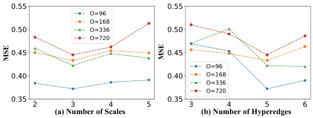
This figure shows the overall framework of the Ada-MSHyper model, which consists of four main modules: Multi-Scale Feature Extraction (MFE), Adaptive Hypergraph Learning (AHL), Multi-Scale Interaction, and Prediction. The MFE module extracts multi-scale feature representations from the input time series. The AHL module learns an adaptive hypergraph structure to model group-wise interactions among the nodes. The Multi-Scale Interaction module captures comprehensive pattern interactions at different scales. Finally, the Prediction module generates predictions based on the learned representations. The figure illustrates the flow of information through each module and highlights the key components of the model.

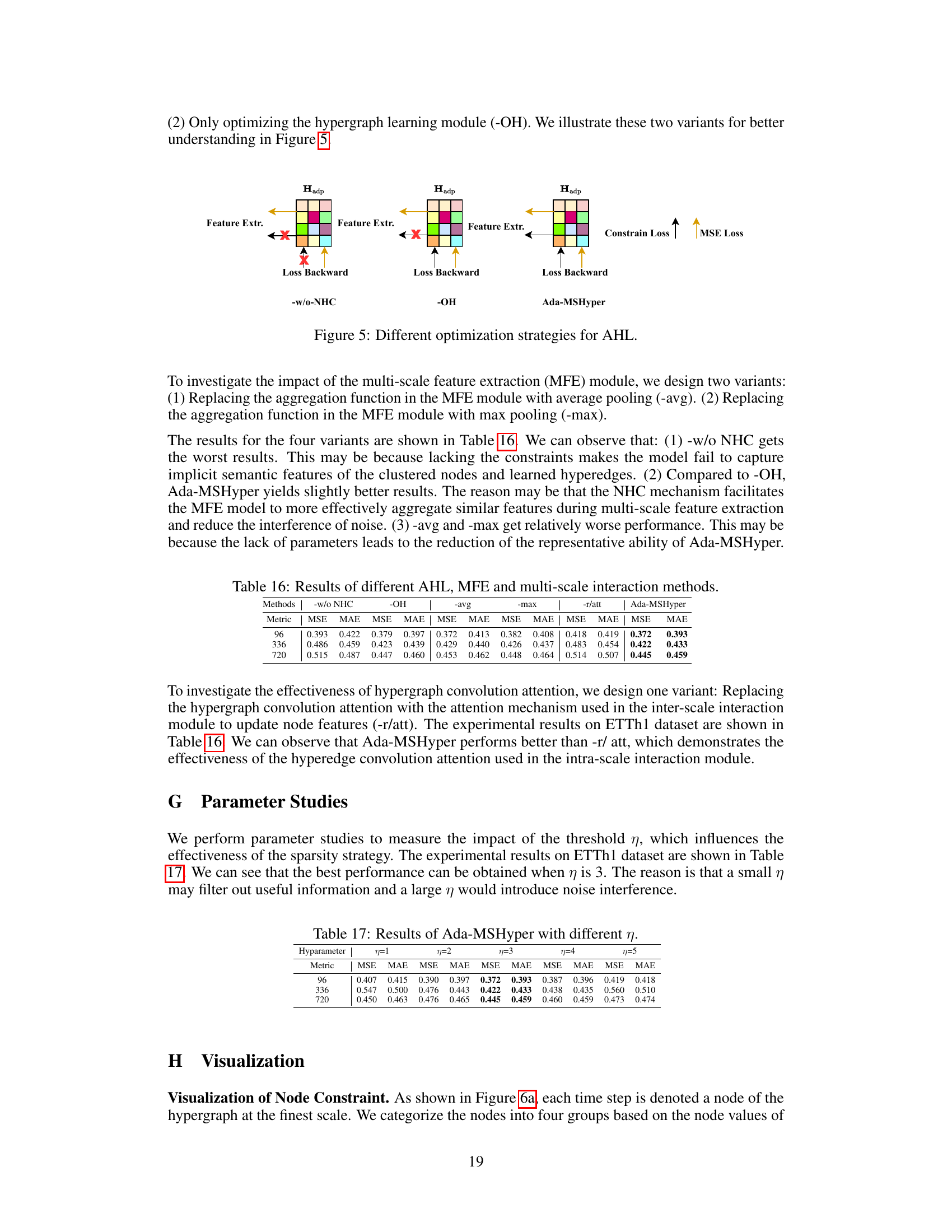
This figure shows three different optimization strategies for the Adaptive Hypergraph Learning (AHL) module. The first, -w/o NHC, shows a basic training process without the node and hyperedge constraints included. The second, -OH, shows only the optimization of the hypergraph learning module itself, without the constraint loss. The final diagram, Ada-MSHyper, represents the complete model which includes both the hypergraph learning and the constraint loss for a complete optimization process.
This figure shows the overall framework of the Ada-MSHyper model, illustrating the four main modules: Multi-Scale Feature Extraction (MFE), Adaptive Hypergraph Learning (AHL), Multi-Scale Interaction, and Prediction. The MFE module processes the input sequence to generate multi-scale feature representations. The AHL module learns an adaptive hypergraph structure to model group-wise interactions. The Multi-Scale Interaction module then utilizes this hypergraph structure to model both intra-scale and inter-scale interactions. Finally, the prediction module generates the final forecasts. The figure also highlights the use of a Node and Hyperedge Constraint (NHC) mechanism within the AHL module to improve the quality of the learned hypergraph.
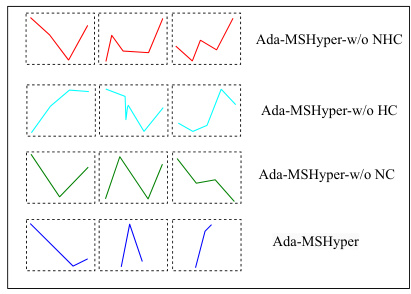
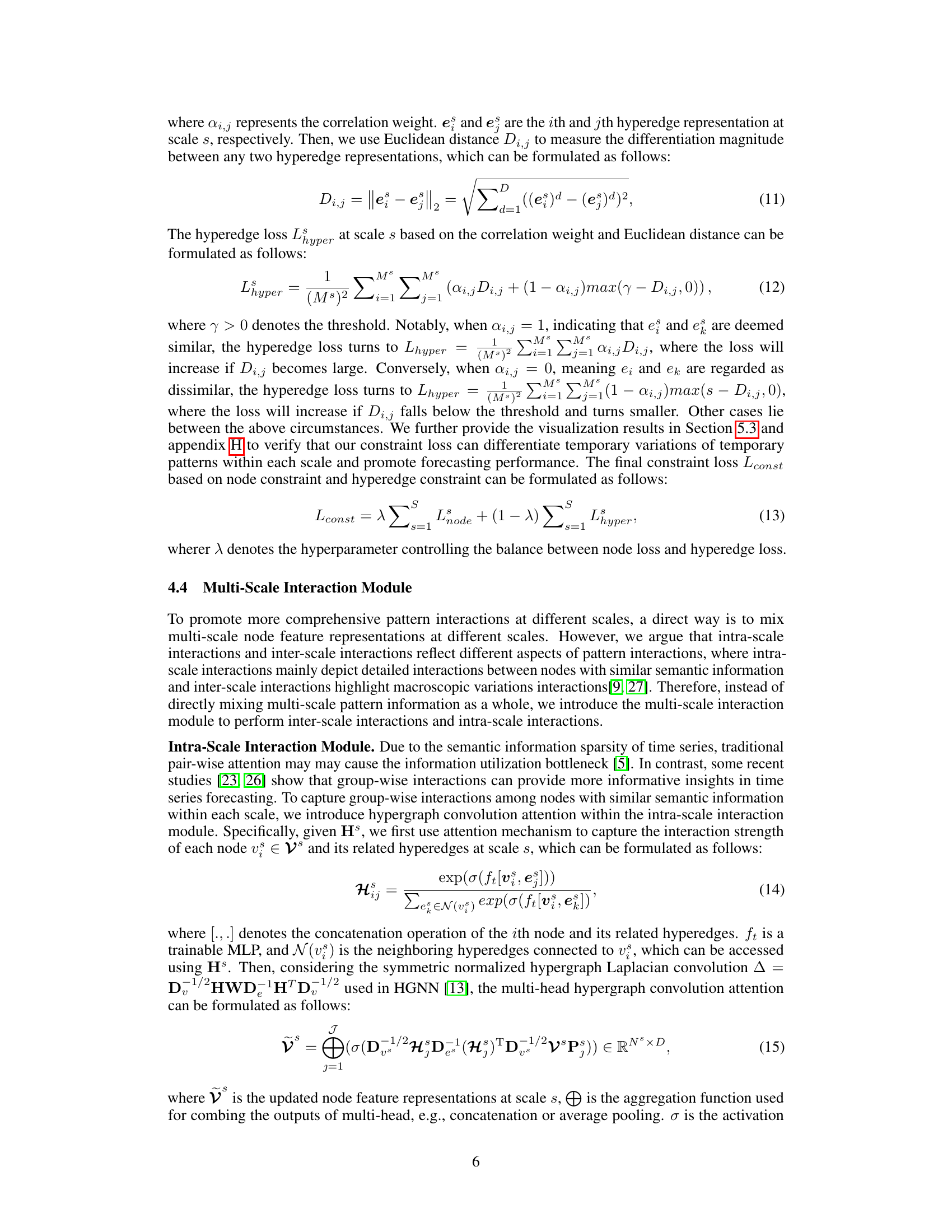
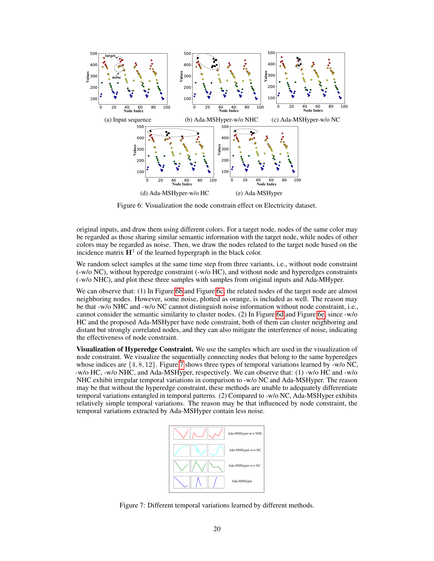
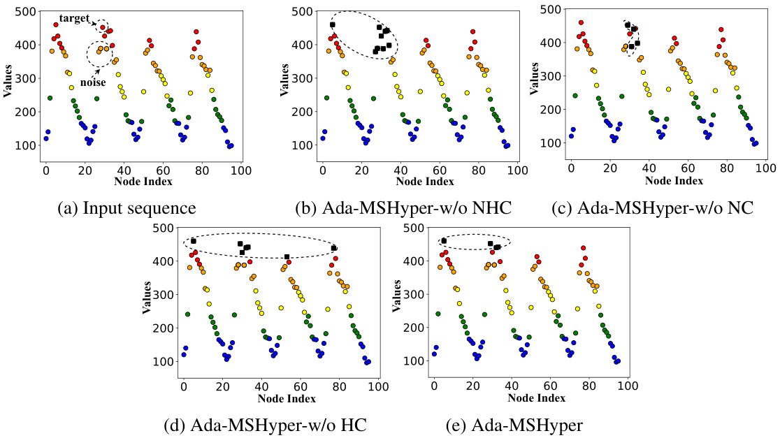
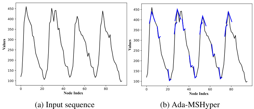
This figure visualizes the impact of node constraints on clustering nodes with similar semantic information. It shows four subfigures: the input sequence, Ada-MSHyper without node constraints (-w/o NHC), Ada-MSHyper without hyperedge constraints (-w/o HC), and Ada-MSHyper. Each subfigure displays the node values at the finest scale, categorized into four groups based on node values. The visualization demonstrates that the node constraint helps cluster nodes with similar semantic information, reducing noise interference, while the hyperedge constraint helps differentiate temporal variations within each scale. The resulting Ada-MSHyper effectively combines both constraints to capture both group-wise semantic information and temporal variations.
The figure shows the overall framework of the proposed Ada-MSHyper model for time series forecasting. It consists of four main modules: (a) Multi-Scale Feature Extraction (MFE) module that extracts feature representations at different scales; (b) Adaptive Hypergraph Learning (AHL) module that automatically generates incidence matrices to model implicit group-wise node interactions; (c) Multi-Scale Interaction Module that performs inter-scale and intra-scale interactions; and (d) Multi-Scale Fusion Module that combines the outputs of multiple scales to generate the final prediction. The diagram visually represents the data flow and interaction between different components of the model.
More on tables

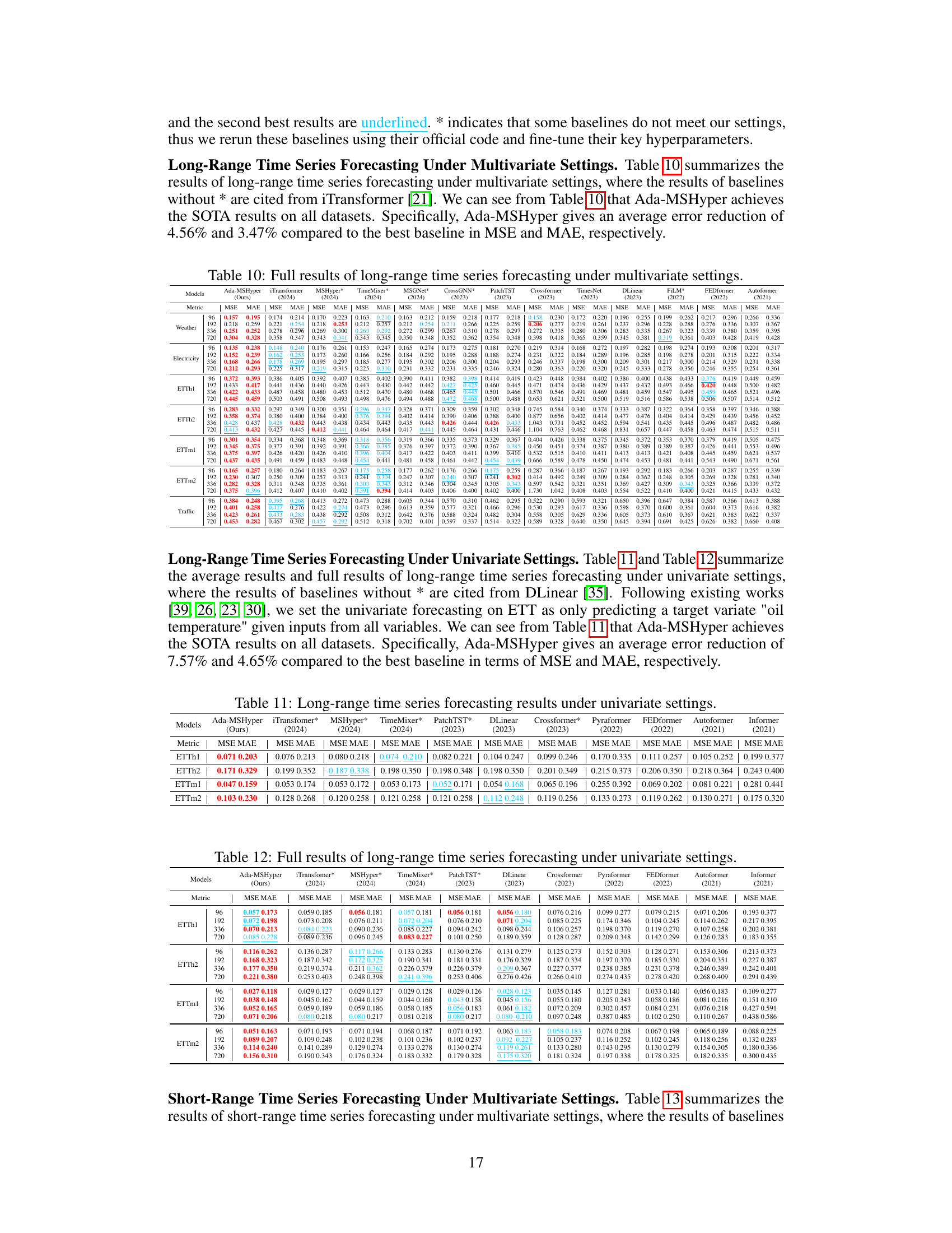
This table presents the complete results for long-range time series forecasting under multivariate settings. It compares the performance of Ada-MSHyper against 13 other methods across multiple datasets and prediction lengths (96, 192, 336, and 720 time steps). The metrics used are Mean Squared Error (MSE) and Mean Absolute Error (MAE). The best-performing method for each dataset and prediction length is highlighted in bold, while the second-best is underlined. The table helps assess the overall effectiveness of Ada-MSHyper compared to existing state-of-the-art approaches.

This table presents the results of short-range time series forecasting experiments conducted under multivariate settings. The results represent the average performance across all prediction lengths tested. The complete results, including individual prediction length results, are detailed in Appendix E. The table compares Ada-MSHyper against several baselines using MSE and MAE metrics.

This table presents the Mean Squared Error (MSE) and Mean Absolute Error (MAE) for long-range time series forecasting using various models, including Ada-MSHyper, under multivariate settings. Results are shown for four different prediction lengths (96, 192, 336, and 720). The table allows for comparison of Ada-MSHyper’s performance against several state-of-the-art baselines across multiple datasets and prediction horizons.

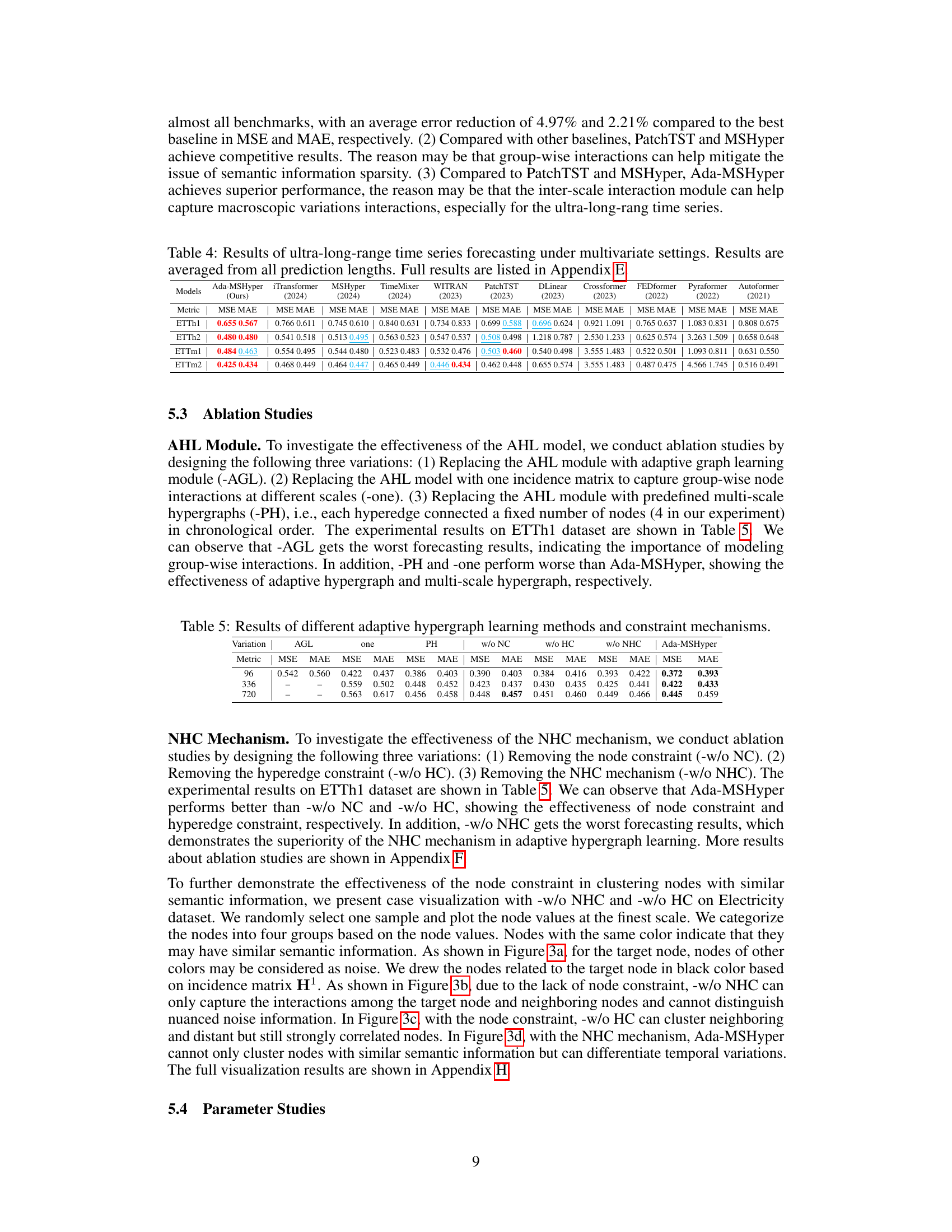
This table presents the results of ablation studies conducted to evaluate the effectiveness of different components of the Ada-MSHyper model. It shows the Mean Squared Error (MSE) and Mean Absolute Error (MAE) for different model variations on the ETTh1 dataset at prediction lengths of 96, 336, and 720. The variations include removing the adaptive graph learning module (-AGL), using a single incidence matrix instead of multiple (-one), using predefined hypergraphs (-PH), removing the node constraint (-w/o NC), removing the hyperedge constraint (-w/o HC), and removing both constraints (-w/o NHC). The table allows for a comparison of these variations against the full Ada-MSHyper model to understand the contribution of each component.

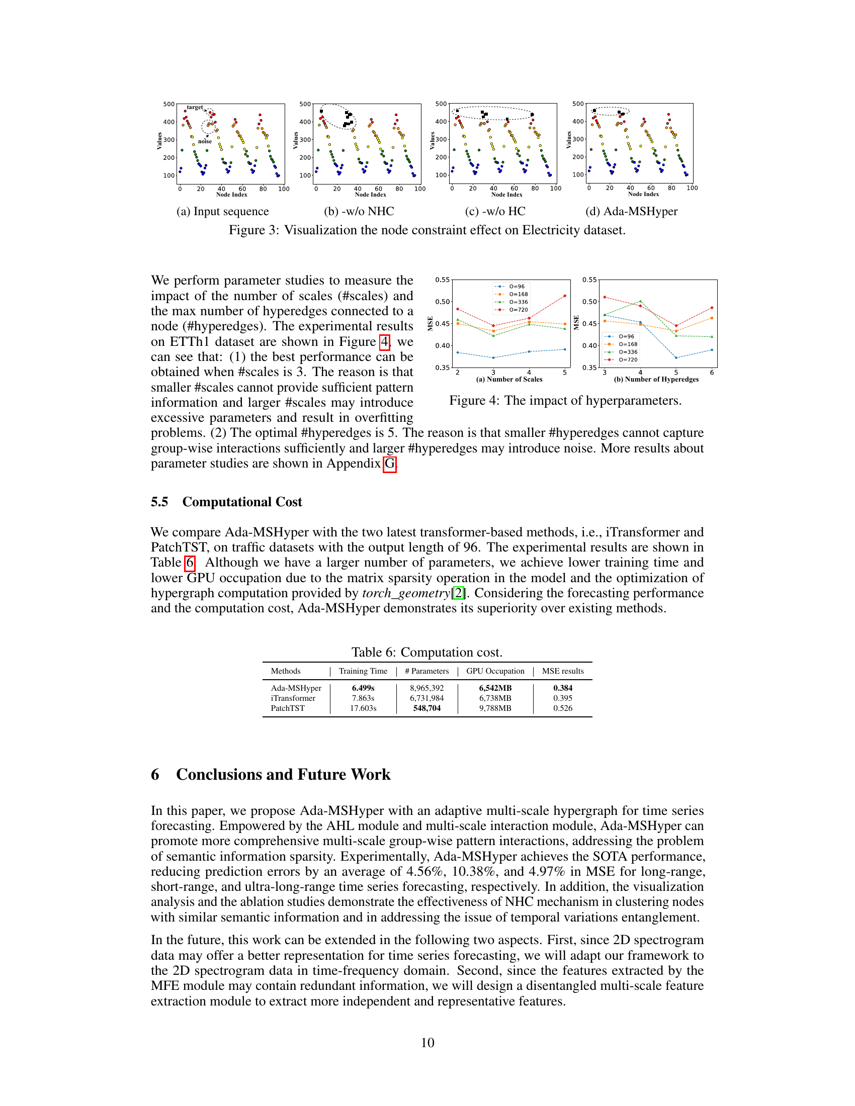
This table compares the computational cost of Ada-MSHyper with two other transformer-based methods (iTransformer and PatchTST) on traffic datasets. The metrics compared are training time, the number of parameters, GPU occupation, and the MSE results. Ada-MSHyper achieves the best MSE result with a comparatively low training time and GPU memory usage despite having a larger number of parameters than iTransformer, but significantly fewer than PatchTST.

This table presents the results of the long-range time series forecasting experiments performed using the Ada-MSHyper model and various baseline models. The results are shown for 7 datasets under multivariate settings, evaluating prediction performance across four prediction lengths. The best and second-best results for each metric (MSE and MAE) are highlighted. A full breakdown of results across all prediction lengths is available in Appendix E.
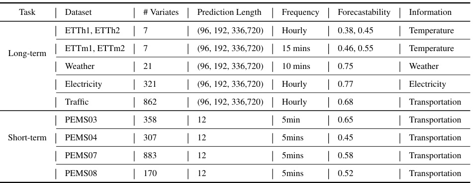
This table provides detailed information on the eleven datasets used in the paper’s experiments. For each dataset, it lists the task (long-term or short-term forecasting), the dataset name, the number of variables, the prediction length(s) considered, the frequency of data collection, the forecastability score (a measure of how predictable the time series is), and the type of information contained in the dataset.
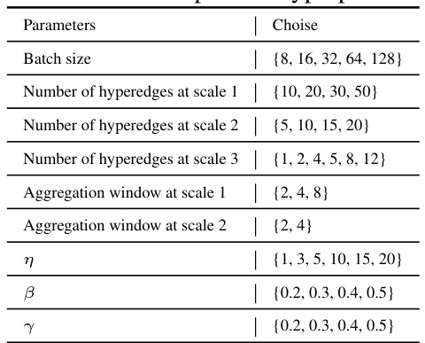
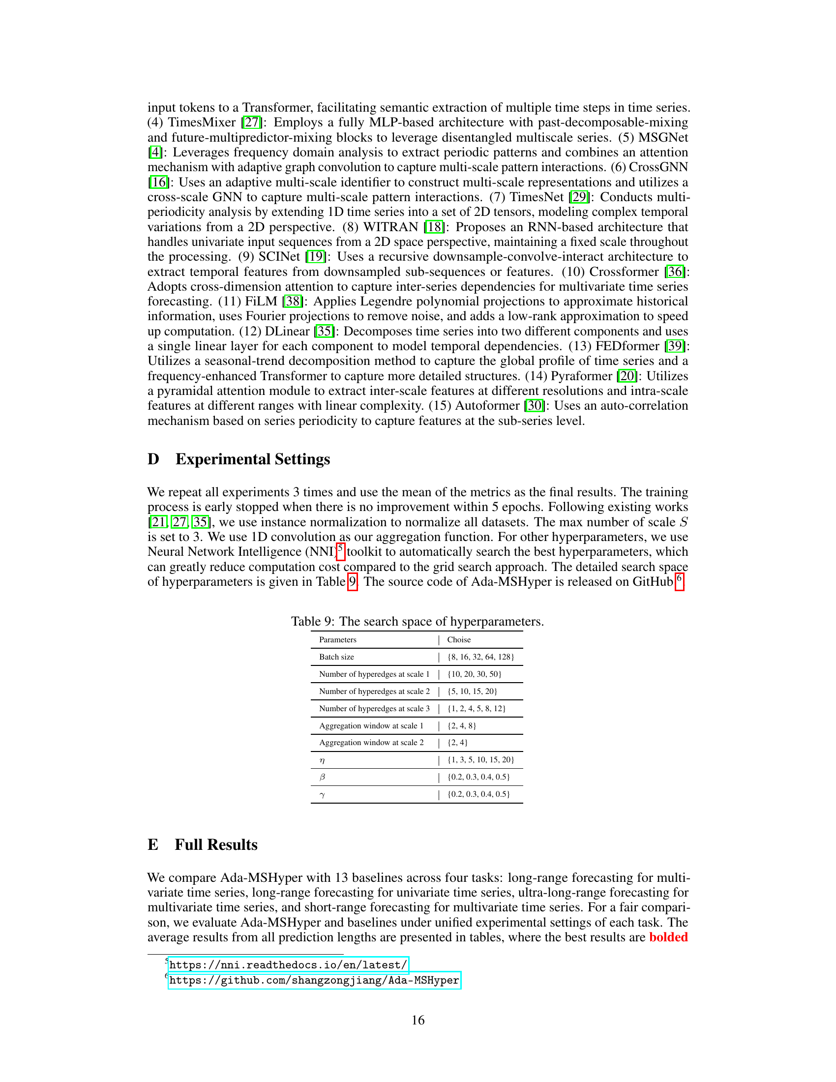
This table presents the range of values considered for each hyperparameter during the hyperparameter search process using the Neural Network Intelligence (NNI) toolkit. The hyperparameters controlled include batch size, the number of hyperedges at each of the three scales, aggregation window sizes at scales 1 and 2, and the threshold parameters η, β, and γ.
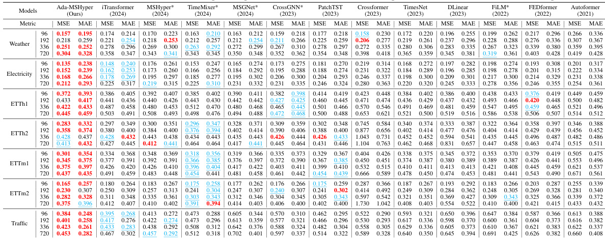
This table presents the complete results of long-range time series forecasting experiments conducted under multivariate settings. It compares the performance of Ada-MSHyper against several baseline methods across multiple datasets and prediction lengths (96, 192, 336, and 720). The metrics used for evaluation are Mean Squared Error (MSE) and Mean Absolute Error (MAE). The table allows for a detailed comparison of Ada-MSHyper’s performance relative to other state-of-the-art models in various forecasting scenarios.

This table presents the complete results for long-range time series forecasting using multiple variables. It compares the performance of Ada-MSHyper against 13 other baselines across four different datasets (Weather, Electricity, ETTh1, ETTh2) and four different prediction lengths (96, 192, 336, 720). The metrics used are MSE (Mean Squared Error) and MAE (Mean Absolute Error), with lower values indicating better performance. The table shows that Ada-MSHyper consistently achieves state-of-the-art results.

This table presents the Mean Squared Error (MSE) and Mean Absolute Error (MAE) for long-range time series forecasting across multiple datasets using Ada-MSHyper and thirteen other baseline methods. The results are shown for four different prediction lengths (96, 192, 336, 720). The table allows for a detailed comparison of Ada-MSHyper’s performance against the state-of-the-art methods on various real-world datasets. The * symbol indicates results taken directly from other papers and not reproduced in the current study.

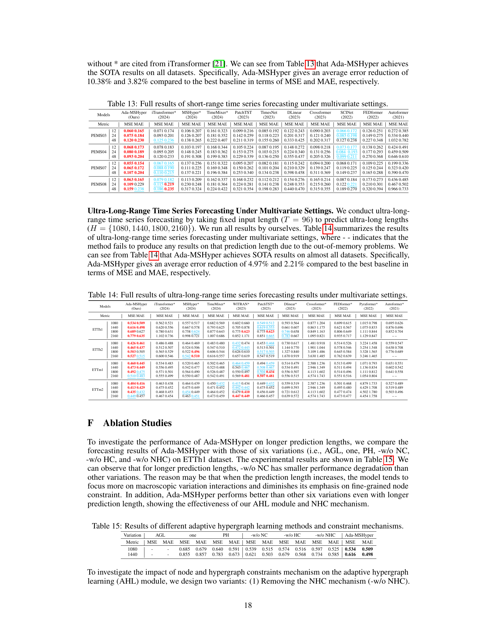
This table presents the results of short-range time series forecasting experiments conducted on four benchmark datasets (PEMS03, PEMS04, PEMS07, and PEMS08) under multivariate settings. The results are averaged over all prediction lengths, and the complete results can be found in Appendix E. The table compares the performance of Ada-MSHyper to several other baseline methods using MSE and MAE metrics.

This table presents a detailed comparison of the proposed Ada-MSHyper model’s performance against 13 baseline models across various metrics (MSE and MAE). It covers four different prediction lengths (96, 192, 336, and 720) for four different datasets (Weather, Electricity, ETTh1, and ETTh2). The results demonstrate the superiority of Ada-MSHyper in achieving state-of-the-art performance on all datasets and prediction lengths.

This table presents the results of ablation studies on the Ada-MSHyper model, comparing its performance against variations where different modules or constraints are removed. The variations include removing the adaptive graph learning module (-AGL), using a single incidence matrix instead of multiple (-one), using predefined multi-scale hypergraphs (-PH), removing the node constraint (-w/o NC), removing the hyperedge constraint (-w/o HC), and removing both constraints (-w/o NHC). The metrics used are MSE and MAE. The results are shown for prediction lengths of 1080 and 1440, demonstrating how the model’s performance changes with different components removed.

This table presents the results of an ablation study comparing different module configurations of Ada-MSHyper, namely removing the node and hyperedge constraint mechanism (-w/o NHC), only optimizing the hypergraph learning module (-OH), replacing the aggregation function in the MFE module with average pooling (-avg) and max pooling (-max), and replacing hypergraph convolution attention with the attention mechanism used in the inter-scale interaction module (-r/att). The results are evaluated using MSE and MAE metrics on the ETTh1 dataset for different prediction lengths (96, 336, and 720). The table shows the impact of each component on the overall performance of Ada-MSHyper.

This table presents the results of Ada-MSHyper using different values for the hyperparameter η, which affects the sparsity of the incidence matrix. The table shows MSE and MAE values for different prediction lengths (96, 336, 720) across five different η values (1, 2, 3, 4, 5). The best performing η value is highlighted, showing the optimal level of sparsity for the model.
Full paper#
