↗ OpenReview ↗ NeurIPS Homepage ↗ Chat
TL;DR#
Time series forecasting (TSF) models often struggle with real-world data due to its non-stationary nature, meaning data distribution changes over time. Existing normalization methods using fixed-time windows cannot effectively capture these complex variations, leading to unreliable predictions. This is a significant limitation for DNN-based TSF methods.
To address this, the paper proposes Dual-domain Dynamic Normalization (DDN), which uses wavelet transforms to decompose time series into different frequencies, then normalizes data in both time and frequency domains using sliding windows. This dynamic approach effectively captures time-varying distribution changes, leading to improved prediction accuracy. Extensive experiments showed that DDN significantly outperforms existing normalization methods when integrated into various forecasting models on multiple benchmark datasets.
Key Takeaways#
Why does it matter?#
This paper is important because it introduces a novel method to improve the accuracy of time series forecasting models, particularly in situations with non-stationary data. The proposed method, Dual-domain Dynamic Normalization (DDN), can be easily integrated into existing forecasting models and has shown significant performance improvements in various benchmark datasets. This makes DDN a valuable tool for researchers working on time series forecasting, opening up new avenues for enhancing the robustness and accuracy of their models. The model-agnostic nature of DDN makes it particularly useful for a wide range of applications.
Visual Insights#
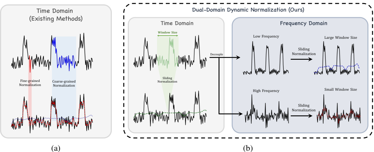
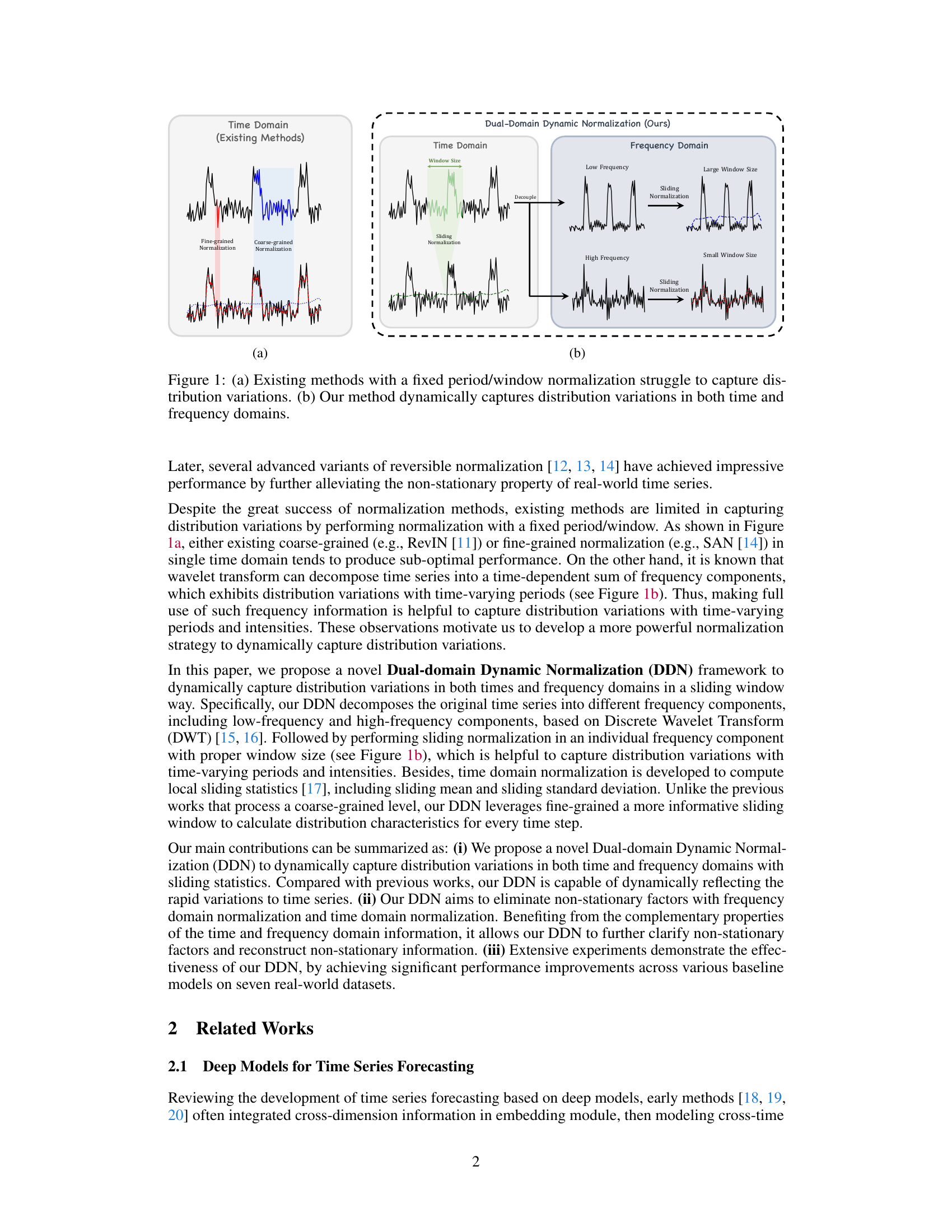
This figure compares existing normalization methods with the proposed Dual-domain Dynamic Normalization (DDN) method. (a) shows how existing methods using a fixed window size for normalization fail to capture distribution variations effectively, especially in dealing with time series data where the distribution changes frequently. (b) illustrates the DDN approach, which dynamically adjusts the window size to adapt to varying distribution patterns in both the time and frequency domains (using wavelet transform to decompose the time series into different frequencies). The DDN approach is designed to achieve better capturing of non-stationary time series characteristics.
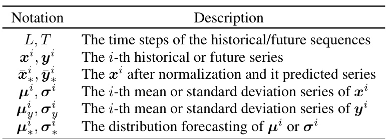
This table compares different methods for handling non-stationarity in time series forecasting. It shows the granularity (series level, input/output level, slice level, point level) at which each method performs normalization and whether the method estimates statistics directly or predicts them.
In-depth insights#
DDN’s Dual-Domain#
The core idea of DDN’s dual-domain approach lies in its ability to capture distribution variations in both the time and frequency domains. Traditional normalization methods often struggle with non-stationary time series, where the data distribution shifts over time, because they only operate in the time domain. DDN addresses this limitation by using the wavelet transform to decompose the time series into different frequency components. This decomposition reveals distribution shifts that might be obscured in the time domain alone, enabling more accurate normalization. By normalizing both the time and frequency domains, DDN provides a more comprehensive and robust way to handle non-stationarity, leading to improved forecasting accuracy. The method’s effectiveness is further enhanced by a sliding window approach, allowing it to adapt to evolving distribution shifts over time. DDN’s modular design makes it easily adaptable to various forecasting models, increasing its versatility and potential impact across various applications.
Dynamic Normalization#
Dynamic normalization methods in time series forecasting aim to address the challenge of non-stationary data, where statistical properties like mean and variance change over time. Traditional normalization techniques often fail because they assume stationarity, leading to inaccurate predictions. Dynamic methods overcome this by adapting the normalization parameters over time, typically using a sliding window approach. This allows the model to focus on recent data with more relevant statistical information for prediction. Key considerations include window size selection—too small may not capture underlying trends, while too large can oversmooth important changes, and the choice of statistics to dynamically compute (e.g., moving averages, rolling standard deviations). The benefits are improved model accuracy and robustness for time series exhibiting distribution shifts and trends. However, limitations exist; computational costs increase, and effective window size and statistic selection are model- and data-dependent. Future research should investigate more sophisticated adaptive techniques and automatic parameter tuning for optimal performance.
Non-Stationarity Tackled#
The concept of tackling non-stationarity in time series forecasting is crucial because real-world data often exhibits significant shifts in its statistical properties over time. Traditional methods that assume stationarity fail in these situations, leading to inaccurate predictions. Addressing this challenge often involves techniques that adapt to these changes. Normalization strategies, for instance, aim to stabilize the data’s distribution, but static normalization may not sufficiently capture dynamic variations. Therefore, dynamic normalization techniques that adjust their parameters based on a sliding window or other adaptive mechanisms are required. Another approach involves incorporating explicit models of distribution changes, either through predicting the distribution directly or using techniques that implicitly learn to represent shifts in statistical properties. Wavelet transforms provide a powerful means of decomposing the time series into different frequency components, separating high and low frequency variations, thus allowing for the flexible modeling of distribution changes across different time scales. Combining techniques, such as wavelet-based decomposition with adaptive normalization, offers a particularly powerful approach, since wavelet transform help to isolate non-stationary aspects while dynamic normalization helps to capture variations.
Benchmark Results#
A dedicated ‘Benchmark Results’ section in a research paper provides crucial insights into the model’s performance. It should present a comparison of the proposed model against established benchmarks or state-of-the-art methods. Quantitative metrics, such as precision, recall, F1-score, accuracy, or MSE, should be clearly reported and analyzed, ideally with statistical significance testing. The choice of metrics should be justified and relevant to the problem domain. A good benchmark analysis also involves a qualitative discussion of results, highlighting strengths and weaknesses. Visualizations, such as graphs or tables, are essential for effective communication of results, allowing for easy comparison of performance across different metrics and models. The discussion should also critically consider the limitations of the benchmarks, potential biases, and the context of the results. Addressing limitations and suggesting future work based on the benchmark results further enhances the section’s value. Overall, a well-structured ‘Benchmark Results’ section demonstrates the model’s capabilities, provides context, and informs future research directions.
Future Research#
Future research directions stemming from this Dual-domain Dynamic Normalization (DDN) for non-stationary time series forecasting could explore several promising avenues. Extending DDN’s applicability to other deep learning architectures beyond the tested models is crucial. Investigating the optimal window size selection for sliding normalization within DDN across various datasets and frequencies merits further study. A potential area for advancement is improving the efficiency of the wavelet transform process within DDN, perhaps through the exploration of alternative wavelet families or optimized algorithms. Moreover, a detailed analysis of DDN’s performance characteristics under different levels of non-stationarity and noise is needed. Finally, research into combining DDN with other advanced time series techniques, such as attention mechanisms or recurrent networks, could lead to even more robust and accurate forecasting models. A comprehensive evaluation on a wider range of real-world datasets representing diverse domains and complexities will strengthen the claims made in this study.
More visual insights#
More on figures
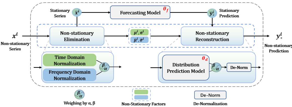
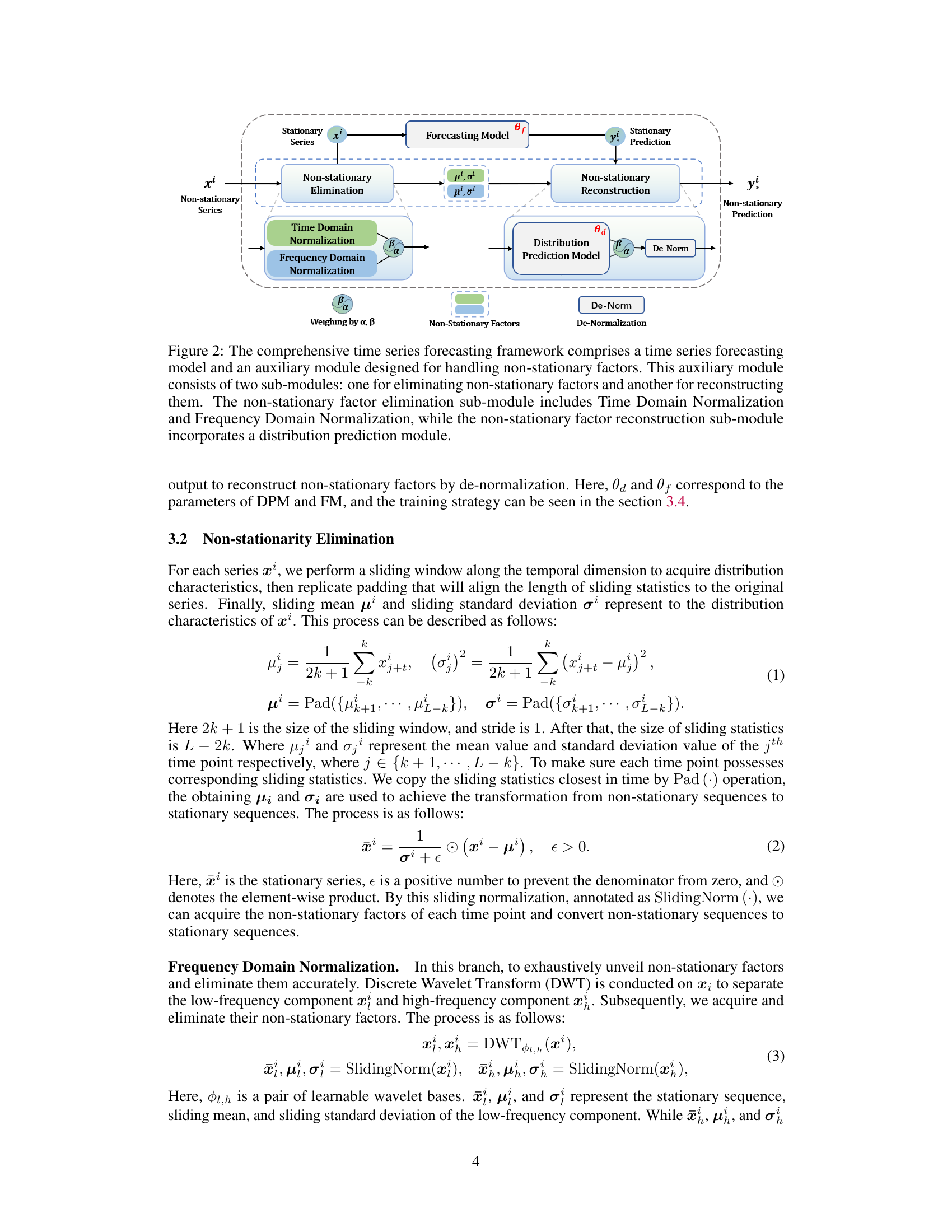
This figure illustrates the overall framework of the Dual-domain Dynamic Normalization (DDN) method for time series forecasting. It shows the two main processing paths: one for the forecasting model itself, and another for handling the non-stationarity of the time series. The non-stationary elimination stage consists of Time Domain Normalization and Frequency Domain Normalization. Then, the non-stationary reconstruction takes the output from the distribution prediction model to reconstruct the non-stationary factors and combine them with the forecasting results to produce a final prediction.
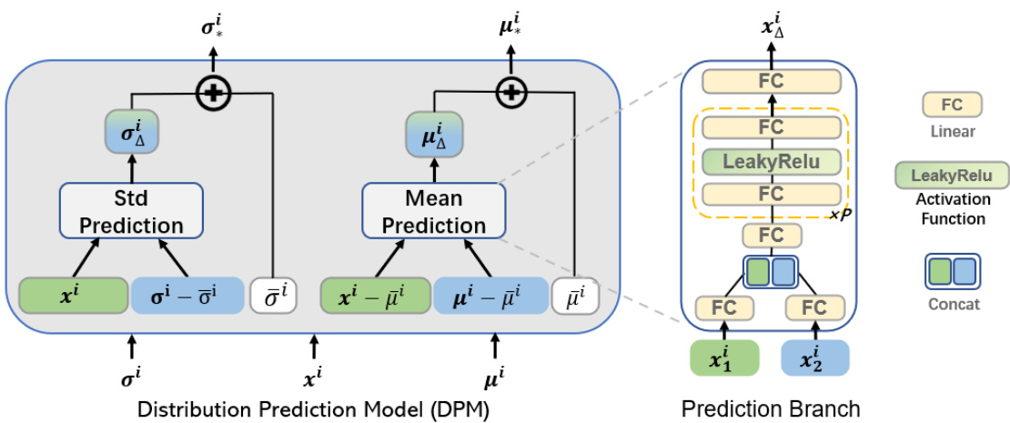
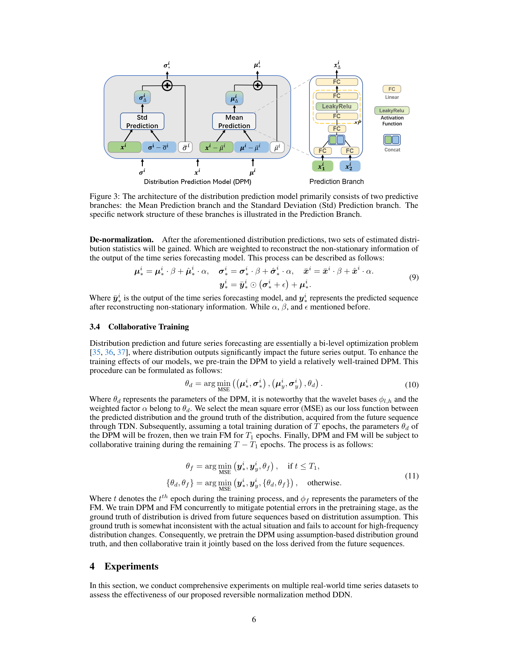
This figure details the architecture of the Distribution Prediction Model (DPM), a key component of the proposed Dual-domain Dynamic Normalization (DDN) framework for time series forecasting. The DPM consists of two main branches: a Mean Prediction branch and a Standard Deviation (Std) Prediction branch. Both branches process input data (xi, μi, σi) to predict future mean (μiΔ) and standard deviation (σiΔ) values, respectively. These branches share a similar network structure, utilizing fully connected (FC) layers, LeakyReLU activation functions, and a concatenation operation to combine intermediate results before the final prediction. The detailed structure of these prediction branches is also illustrated in the figure.

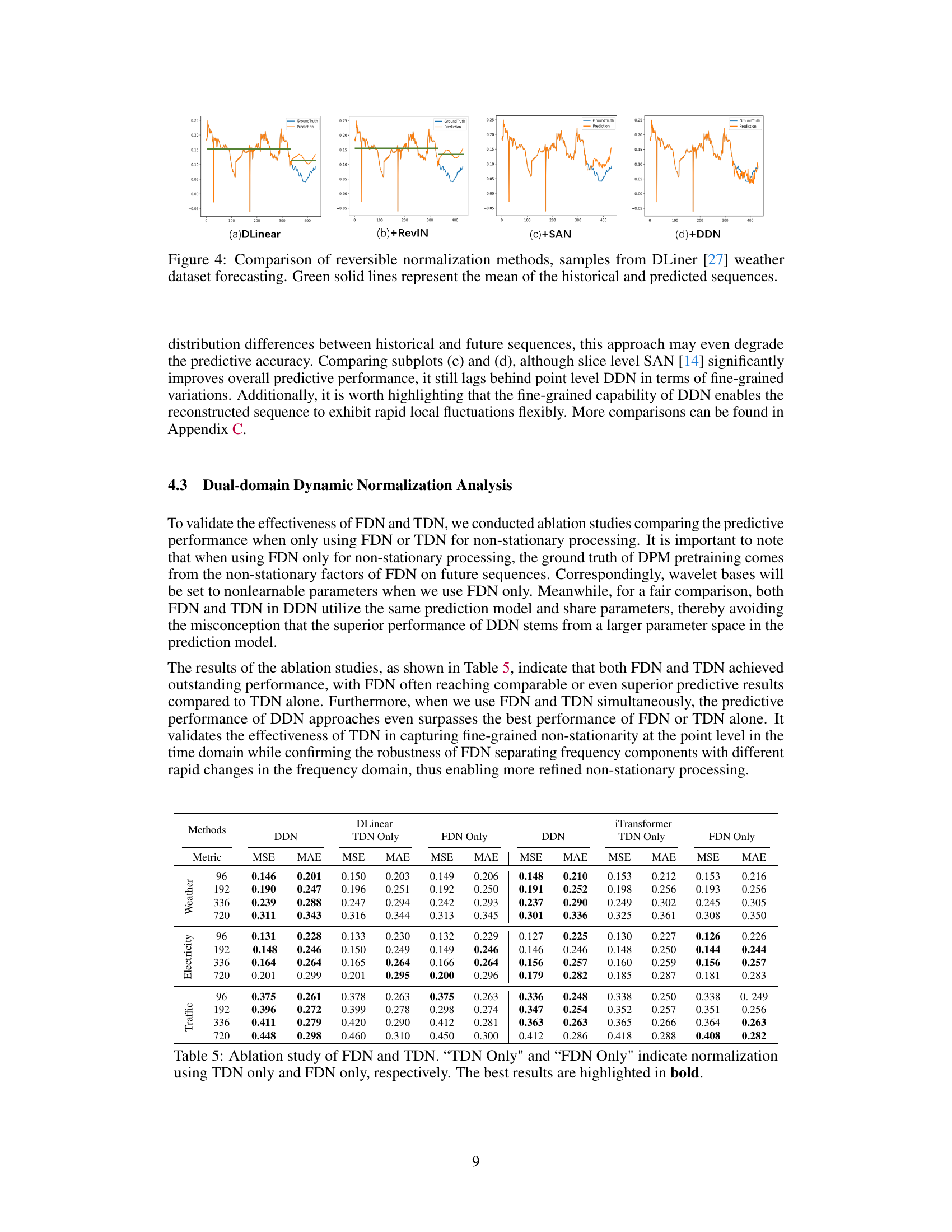
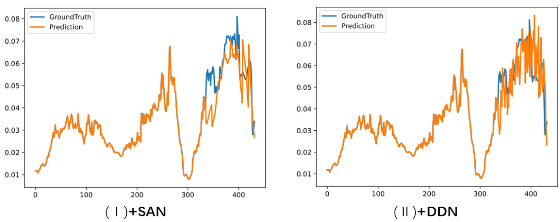
This figure compares four different reversible normalization methods: DLinear, DLinear+RevIN, DLinear+SAN, and DLinear+DDN. Each method’s performance is visualized by plotting its predictions (orange line) against the ground truth (blue line) for a sample from the DLiner weather dataset forecast. The green line represents the mean values of both the historical and predicted sequences for easier comparison and understanding of the differences between the methods.
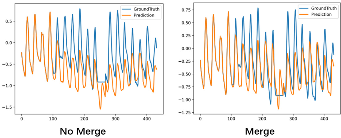
This figure compares the performance of NST with and without merging the non-stationary factors extraction module into the feature. The left panel shows the results without merging, while the right panel shows the results with merging. The results show that merging the non-stationary factors extraction module into the feature improves the performance of NST.

This figure compares the performance of four different reversible normalization methods (DLinear, DLinear+RevIN, DLinear+SAN, and DLinear+DDN) on the Weather dataset using the DLiner model. The green solid lines represent the means of the historical and predicted sequences. The figure shows that the DDN method is the only method that accurately captures the distribution variations of the real-world data, exhibiting better performance in terms of prediction accuracy and dynamic adaptability compared to other methods.

This figure compares the performance of four different reversible normalization methods (DLinear, DLinear+RevIN, DLinear+SAN, and DLinear+DDN) on a weather forecasting task using the DLinear model. The green lines represent the mean of the historical and predicted sequences, illustrating how each method handles the non-stationary nature of the data. The figure shows that DDN (Dual-domain Dynamic Normalization) outperforms the other methods, achieving a prediction that aligns more closely with the actual values. The differences highlight the effectiveness of DDN in capturing distribution variations compared to other reversible normalization methods.

This figure compares four different reversible normalization methods (DLinear, RevIN, SAN, and DDN) applied to the weather dataset using the DLiner model. The plots show the predicted values against the ground truth. The goal is to visually illustrate the differences in how each method handles distribution shifts and reconstructs non-stationary information in time series forecasting. The green lines show the average of the historical and predicted values. This helps assess how each method aligns the predicted and actual distribution of the time series.
This figure compares the performance of NST (Non-stationary transformer) model with and without merging non-stationary factors extraction module. The results show that merging this module improves the performance of the model.
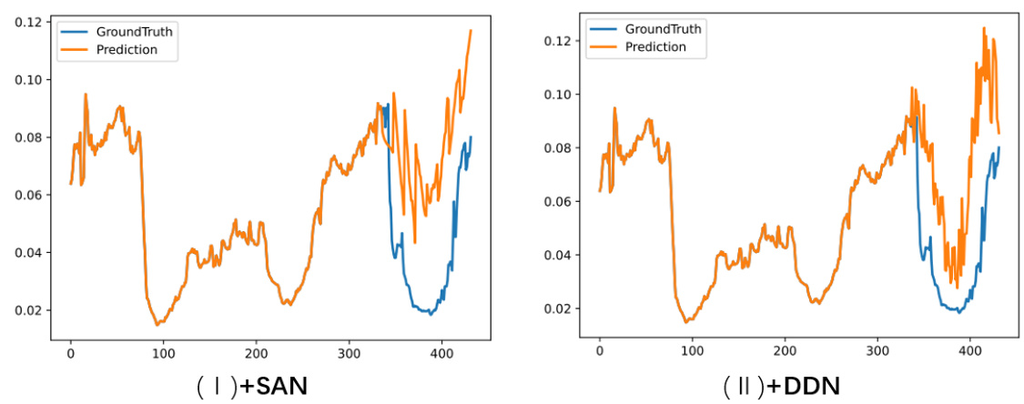
This figure compares four different reversible normalization methods applied to weather forecasting using the DLinear model. It visually demonstrates how well each method captures the distribution of the time series. The original time series (ground truth) is shown in blue, and the predictions for each method are shown in orange. The green line represents the mean. By comparing the orange prediction lines to the blue ground truth, the relative strengths and weaknesses of each normalization method in terms of capturing dynamic changes in the data can be seen.
This figure illustrates the difference between existing normalization methods and the proposed Dual-domain Dynamic Normalization (DDN) method in capturing distribution variations in time series forecasting. Panel (a) shows how traditional methods with fixed-size windows fail to adapt to changes in data distribution across time. Panel (b) demonstrates how DDN overcomes this limitation by dynamically capturing variations in both the time domain and the frequency domain (using wavelet transforms), enabling more accurate modeling of complex temporal patterns.
More on tables

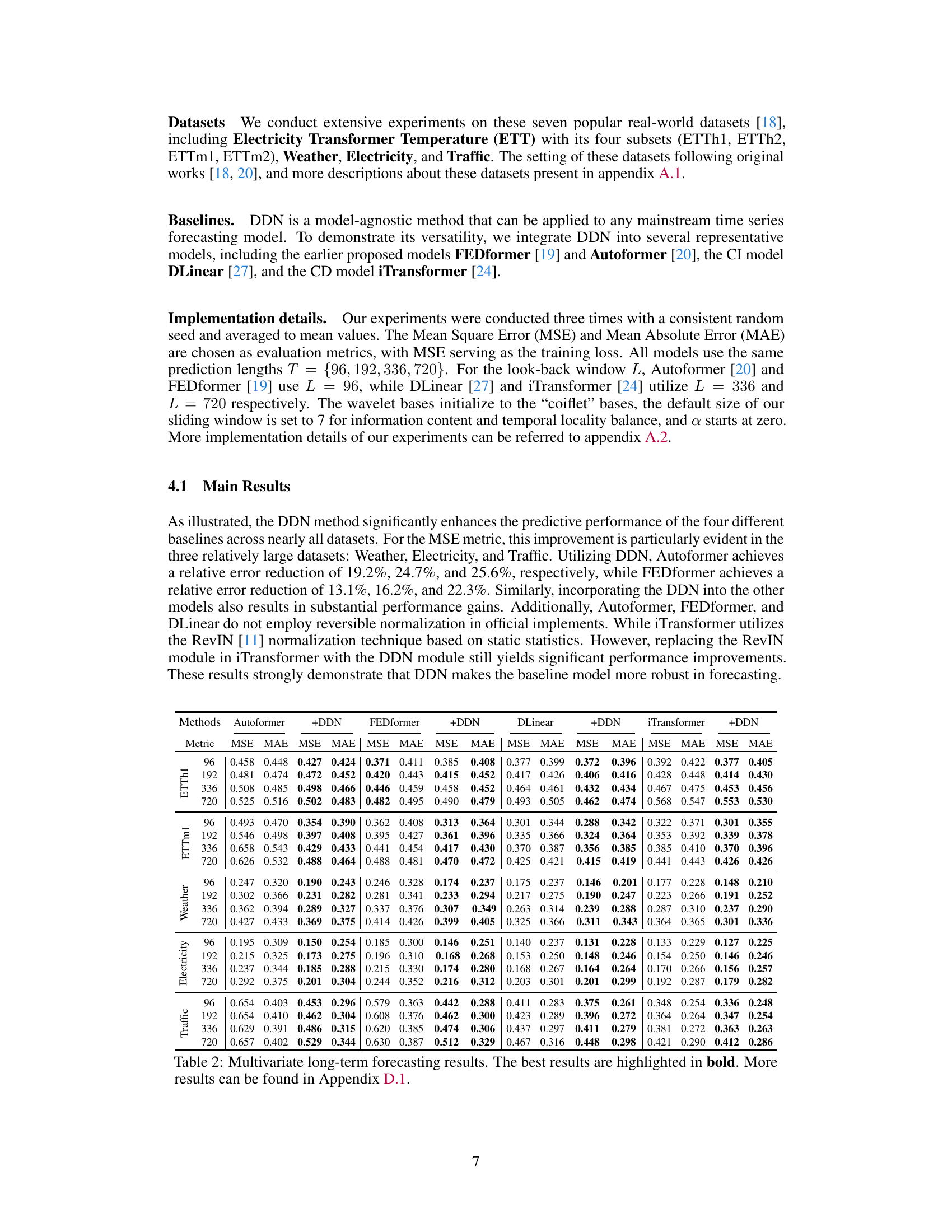
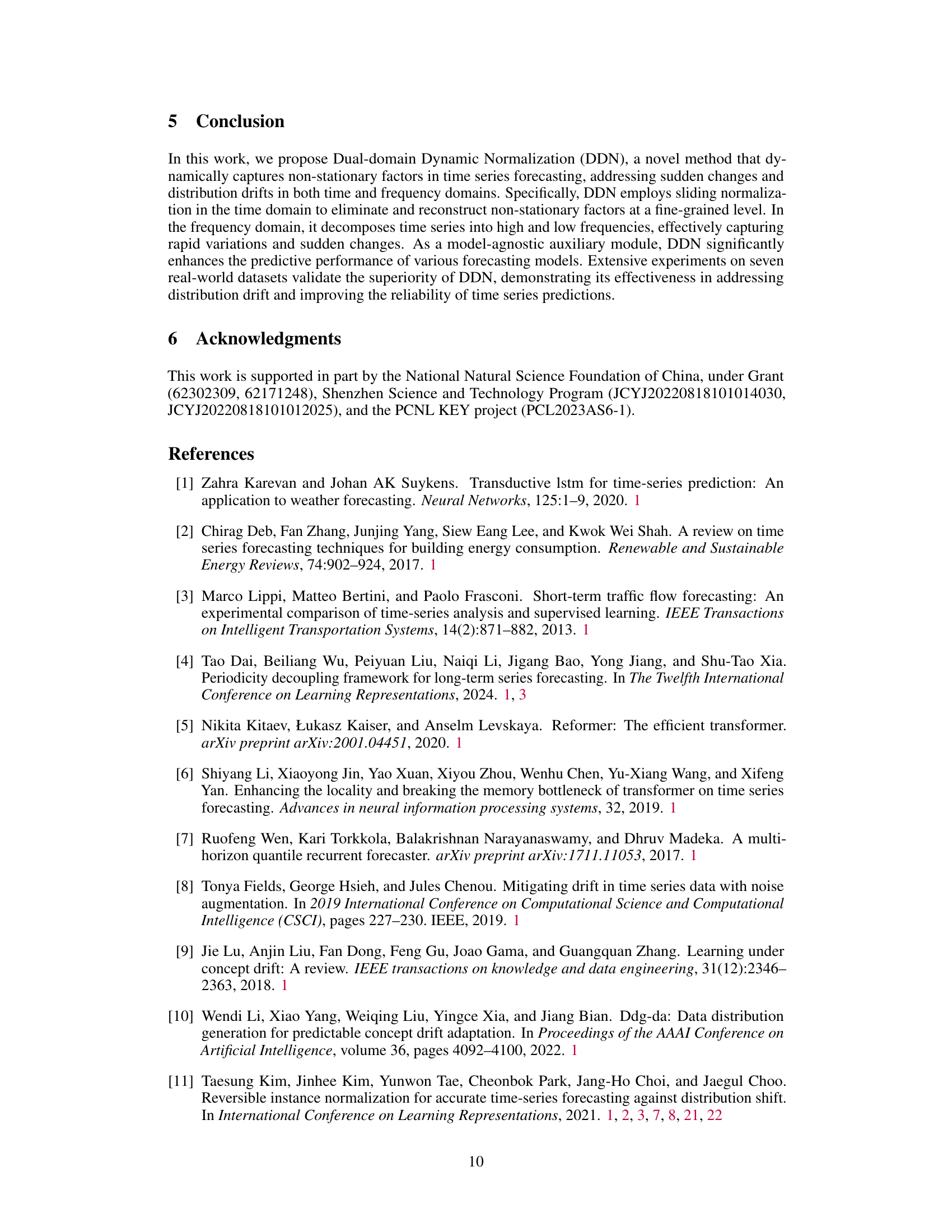
This table presents the results of long-term multivariate time series forecasting experiments using four different models (Autoformer, FEDformer, DLinear, and iTransformer), each with and without the proposed DDN method. The results are shown for four different prediction lengths (T = 96, 192, 336, 720) and across seven datasets (ETTh1, ETTh2, ETTm1, ETTm2, Weather, Electricity, and Traffic). The best-performing model for each combination of dataset and prediction length is highlighted in bold. More detailed results are available in Appendix D.1.

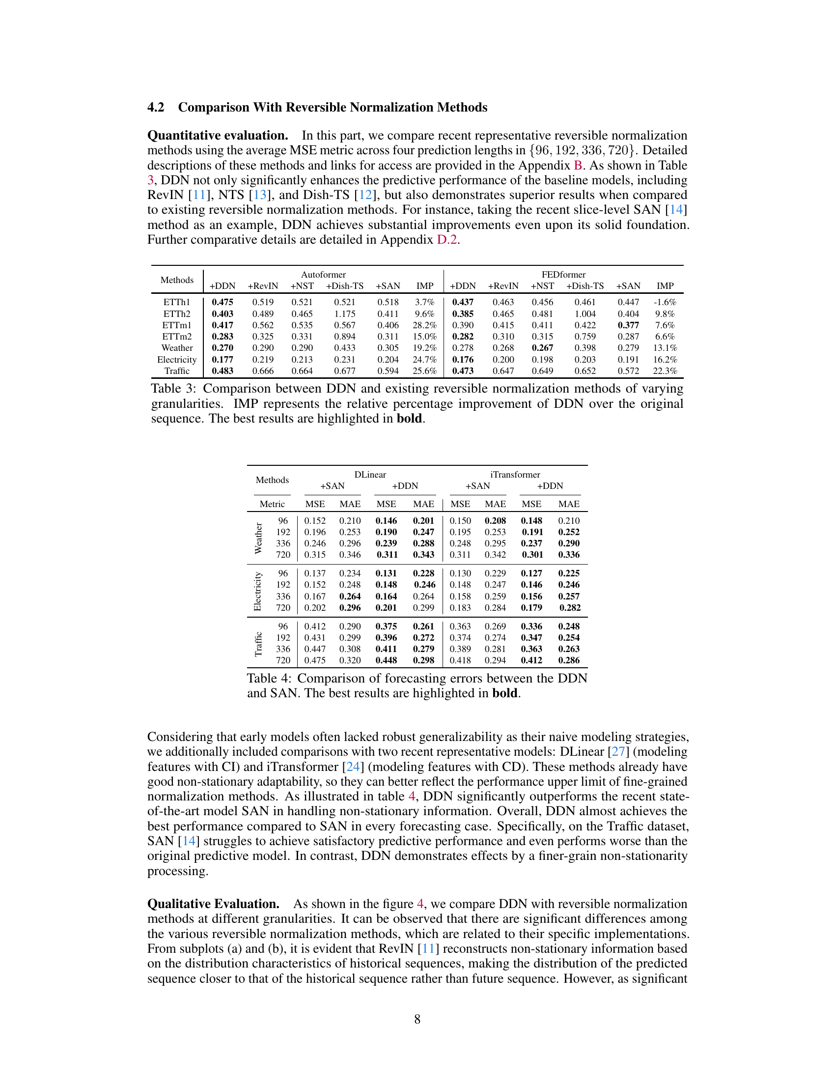
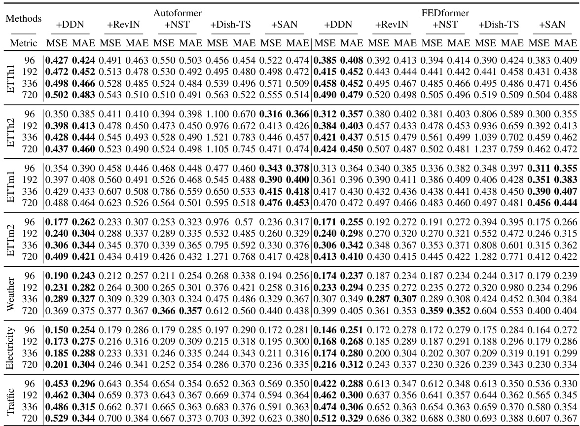
This table compares the performance of the proposed Dual-domain Dynamic Normalization (DDN) method against other existing reversible normalization methods (RevIN, NST, Dish-TS, SAN). The comparison is done across multiple datasets (ETTh1, ETTh2, ETTm1, ETTm2, Weather, Electricity, Traffic) and considers various prediction lengths. The ‘IMP’ column indicates the percentage improvement of DDN over the original method, highlighting the effectiveness of DDN in improving forecasting accuracy.
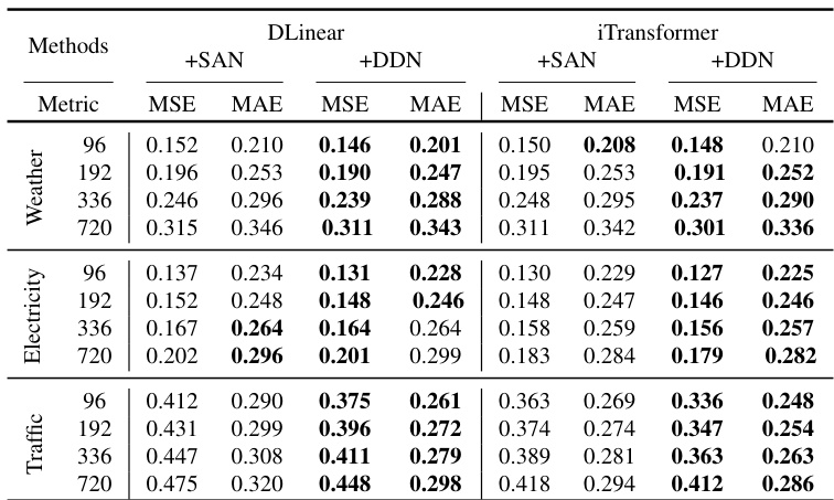
This table compares the performance of the proposed Dual-domain Dynamic Normalization (DDN) method against other existing reversible normalization methods, namely RevIN, NST, Dish-TS, and SAN. The comparison is done across multiple datasets (ETTh1, ETTh2, ETTm1, ETTm2, Weather, Electricity, Traffic) and uses two evaluation metrics (MSE and MAE). The ‘IMP’ column shows the percentage improvement achieved by DDN over the original method for each dataset and metric. The best results for each setting are highlighted in bold, demonstrating DDN’s superior performance.

This table compares different methods for handling non-stationary time series data in forecasting. It shows the granularity (how finely the data is normalized) and the method used to estimate the non-stationary parameters for each approach. This helps to understand the differences in how these methods handle the changing distribution characteristics of non-stationary time series. It includes methods like RevIN, NST, Dish-TS, SAN, and the proposed DDN.
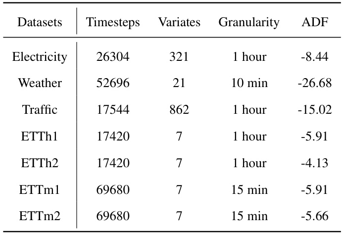
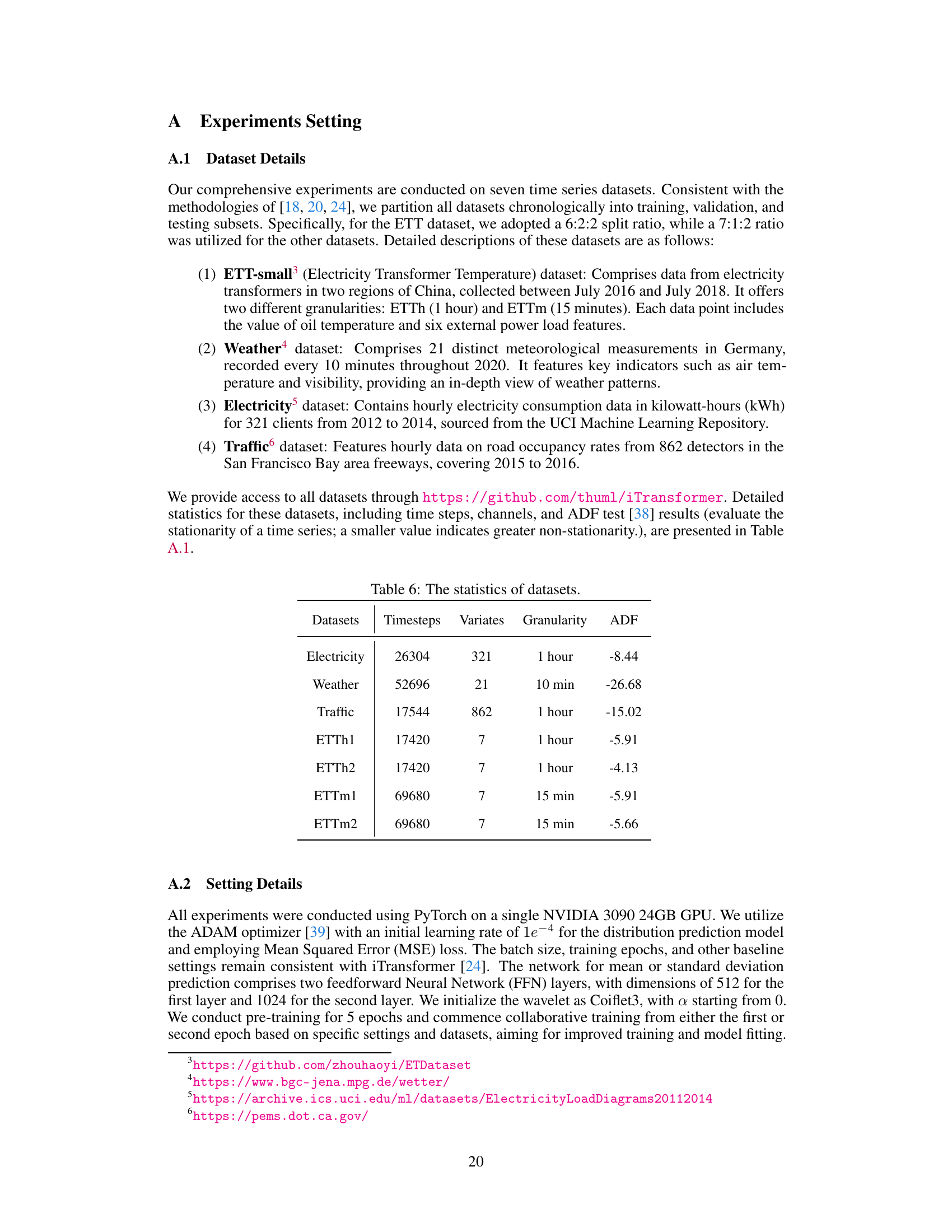
This table provides a summary of the seven time series datasets used in the paper’s experiments. For each dataset, it lists the number of timesteps, the number of variates (or channels), the granularity of the data (e.g., 1 hour, 10 minutes), and the Augmented Dickey-Fuller (ADF) test statistic. The ADF statistic is a measure of stationarity, with lower values indicating greater non-stationarity.

This table compares five different reversible normalization methods: RevIN, NST, Dish-TS, SAN, and DDN (the proposed method). It contrasts their approaches to handling non-stationarity in time series forecasting by categorizing them based on two key aspects: the granularity of their normalization (series level, input/output level, slice level, or point level) and the method used for estimating the non-stationary components (statistics or prediction). The table helps to illustrate the evolution and relative sophistication of techniques for addressing non-stationarity in forecasting.
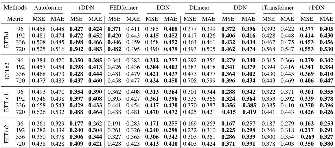
This table presents the results of multivariate long-term time series forecasting experiments using four different models (Autoformer, FEDformer, DLinear, and iTransformer), each combined with the proposed Dual-domain Dynamic Normalization (DDN) method. The results are shown for four different prediction lengths (96, 192, 336, and 720) and are evaluated using Mean Squared Error (MSE) and Mean Absolute Error (MAE). The best performance for each model and prediction length is highlighted in bold. More detailed results are available in Appendix D.1.
This table presents the results of long-term multivariate time series forecasting experiments using four different deep learning models (Autoformer, FEDformer, DLinear, and iTransformer) with and without the proposed Dual-domain Dynamic Normalization (DDN) method. The models were evaluated on seven real-world datasets (ETTh1, ETTh2, ETTm1, ETTm2, Weather, Electricity, and Traffic) using mean squared error (MSE) and mean absolute error (MAE) metrics and different prediction lengths (T=96, 192, 336, 720). The best performance for each model and dataset is highlighted in bold. Further details are available in Appendix D.1.
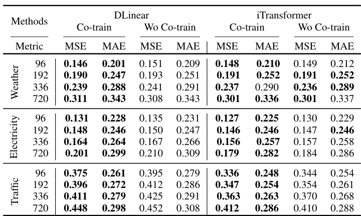
This table presents the Mean Squared Error (MSE) and Mean Absolute Error (MAE) for four different forecasting models (Autoformer, FEDformer, DLinear, and iTransformer) on seven real-world datasets (ETTh1, ETTh2, ETTm1, ETTm2, Weather, Electricity, and Traffic). The results are shown for four different prediction lengths (96, 192, 336, and 720). The best performance for each model and dataset is highlighted in bold. More detailed results are available in Appendix D.1.
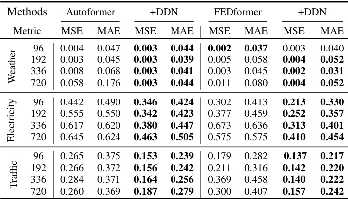
This table presents the results of multivariate long-term time series forecasting experiments using different models (Autoformer, FEDformer, DLinear, iTransformer) with and without the proposed Dual-domain Dynamic Normalization (DDN) method. It shows Mean Squared Error (MSE) and Mean Absolute Error (MAE) for four different prediction lengths (96, 192, 336, 720) across seven datasets (ETTh1, ETTh2, ETTm1, ETTm2, Weather, Electricity, Traffic). The best performance for each model and prediction length is highlighted in bold. Additional details are available in Appendix D.1.
Full paper#
