Statistical and Geometrical properties of the Kernel Kullback-Leibler divergence

↗ OpenReview ↗ NeurIPS Homepage ↗ Chat

TL;DR

#

Key Takeaways

#

Why does it matter?

#

This paper is important as it introduces a regularized version of the Kernel Kullback-Leibler (KKL) divergence, addressing limitations of the original KKL. This leads to improved applicability, especially for discrete distributions, and offers a novel approach for comparing probability distributions in machine learning. The closed-form solution and efficient optimization algorithm make it practically useful. It opens avenues for improved generative modeling and Bayesian inference.

Visual Insights

#

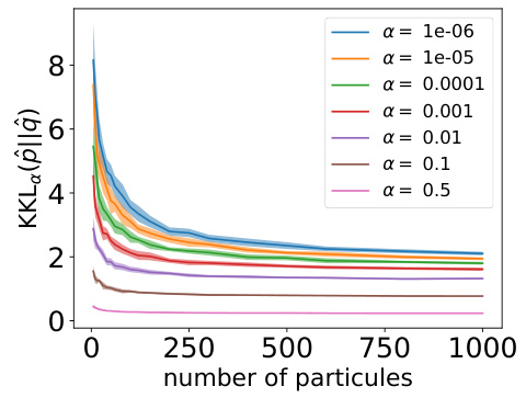
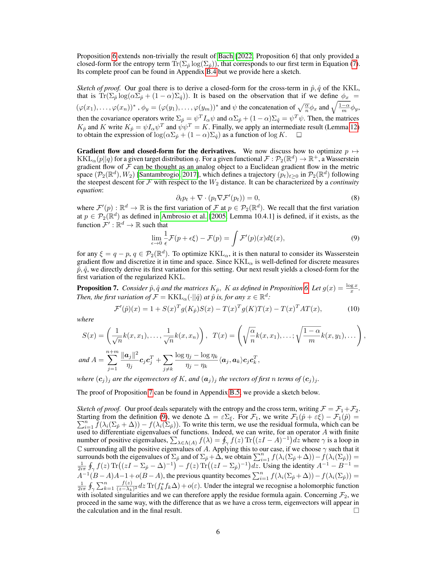
This figure shows the concentration of the regularized Kernel Kullback-Leibler (KKL) divergence around its population limit as the number of samples increases. The experiment uses two anisotropic Gaussian distributions (p and q) in 10 dimensions. The plot displays the empirical KKL (KKLɑ(p̂, q̂)) for different values of the regularization parameter α. The results are averaged over 50 runs, showing the mean and standard deviation. The figure demonstrates that the empirical KKL converges to its population value faster as α increases.

In-depth insights

#

Regularized KKL

#

The core concept of “Regularized KKL” centers on addressing the limitations of the original Kernel Kullback-Leibler (KKL) divergence. The original KKL, while offering advantages in comparing probability distributions through kernel embeddings, suffers from being undefined for distributions with disjoint supports. Regularization, achieved by a mixture of the distributions (αp + (1-α)q), ensures the divergence remains well-defined. This modification allows for analysis of a broader range of distributions, expanding the applicability of KKL. The paper further investigates the properties of this regularized variant, deriving bounds to quantify the deviation from the original KKL and establishing finite-sample guarantees. This detailed analysis, complemented by closed-form expressions for discrete distributions and a Wasserstein gradient descent scheme, makes the regularized KKL a practical and theoretically sound tool for machine learning tasks involving the approximation or transport of probability distributions.

KKL Gradient Flow

#

The concept of “KKL Gradient Flow” centers on using the regularized kernel Kullback-Leibler (KKL) divergence as an objective function to guide the iterative optimization of probability distributions. This approach leverages the strengths of KKL, which unlike traditional KL divergence, remains well-defined even for distributions with disjoint support, thanks to a novel regularization technique. The gradient flow method allows for a smooth transition between distributions, unlike other methods which might suffer from abrupt changes or instability. The closed-form expressions for the regularized KKL and its gradient are crucial for implementing efficient optimization schemes like Wasserstein gradient descent, making the proposed methodology computationally feasible. The core strength lies in its ability to approximate the target distribution q effectively, and gracefully handles cases where standard methods falter. Empirical results demonstrate improved convergence properties compared to standard techniques, highlighting the potential of KKL Gradient Flow as a valuable tool in machine learning applications where approximating a target distribution is paramount.

KKL Closed-Form

#

The subsection on “KKL Closed-Form” is crucial because it bridges the gap between the theoretical formulation of the regularized Kernel Kullback-Leibler (KKL) divergence and its practical implementation. The authors demonstrate that for discrete probability distributions, the regularized KKL can be expressed in a closed form using kernel Gram matrices. This is a significant contribution because it avoids computationally expensive iterative methods often needed for divergence calculations. The closed-form expression enables efficient computation of the KKL and its derivatives, paving the way for practical optimization algorithms such as Wasserstein gradient descent. This closed-form expression, specifically tailored for discrete distributions which are common in machine learning applications, is a major step toward making the KKL a viable alternative to other common divergences. The efficient computability makes the proposed regularized KKL a practical tool for various machine learning tasks, such as distribution approximation and generative modeling.

Finite Sample Bds

#

In statistical learning, establishing finite sample bounds is crucial for understanding the performance of an estimator or algorithm in practice. These bounds provide guarantees on the accuracy or error of the method, given a finite amount of training data. For the regularized KKL divergence, finite sample bounds would quantify how well the estimated divergence from finite samples approximates the true divergence. Such bounds would be particularly important to determine the number of samples needed for a reliable estimate and to understand the impact of regularization on the estimator’s behavior. They would ideally provide high-probability statements about the deviation between the estimated and true regularized KKL divergence, potentially depending on properties of the underlying probability distributions and the kernel function. The tightness of these bounds would also be a key factor in their practical utility. A sufficiently tight bound would enable the determination of realistic sample sizes needed for practical applications, while loose bounds would be less informative.

Empirical Results

#

An ‘Empirical Results’ section in a research paper would present the findings of experiments conducted to validate the paper’s claims. A strong section would begin by clearly stating the experimental setup, including datasets, parameter settings, and evaluation metrics. Results should be presented visually (e.g., graphs, tables) and numerically (e.g., precision, recall, F1-score), facilitating easy comprehension. Crucially, it should highlight key trends, comparing proposed methods against baselines to show significant improvements or any unexpected behavior. Statistical significance of the results (e.g., p-values, confidence intervals) should be rigorously reported, demonstrating the reliability of the findings and minimizing the possibility of spurious correlations. A thoughtful discussion of the results, acknowledging limitations and potential biases, would strengthen the section, offering insights into the broader implications of the work and suggesting directions for future research. Reproducibility is vital, ensuring that sufficient detail is included for other researchers to repeat the experiments and verify the findings. Omitting any of these elements would undermine the credibility and impact of the paper.

More visual insights

#

More on figures

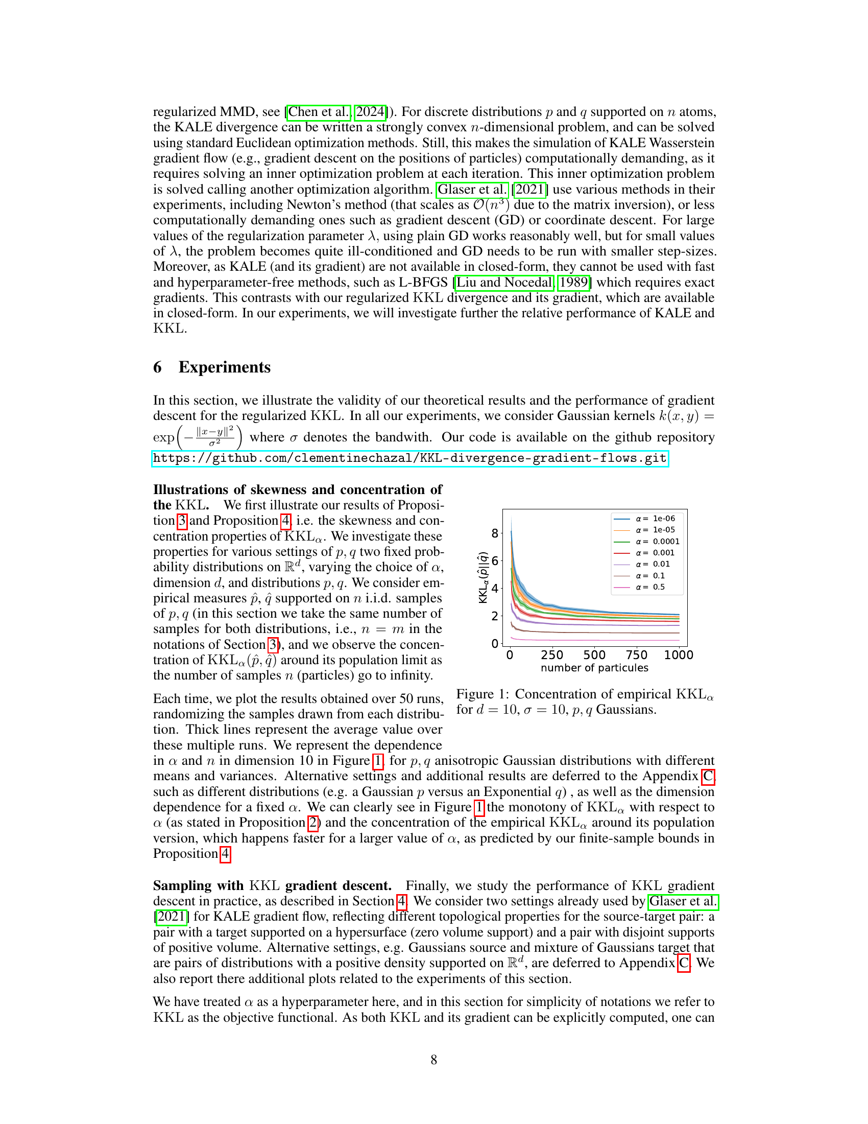
This figure compares the performance of three different gradient flows (MMD, KALE, and KKL) in transporting a set of points to a target distribution shaped as three non-overlapping rings. The images show the evolution of the point cloud at different time steps during the optimization process. It visualizes how each method’s gradient flow affects the distribution of the points over time. The figure highlights the strengths and weaknesses of each approach in terms of approximating the target distribution.

The figure illustrates the concentration of the regularized Kernel Kullback-Leibler (KKL) divergence for empirical measures around its population limit as the number of samples increases. It shows the results obtained over 50 runs for different values of the regularization parameter α, with thick lines representing the average values. The distributions p and q are anisotropic Gaussian distributions with different means and variances. The figure demonstrates the convergence behavior of the empirical KKL towards its population counterpart, which is faster for larger values of α as predicted by the theoretical results.

This figure displays the evolution of the 2-Wasserstein distance (W2(p||q)) during the gradient descent in dimension d=10 for various parameters α. The initial distribution p is a Gaussian, and the target distribution q is a mixture of two Gaussians. The plot shows the average W2(p,q) over 10 runs, where the mean of p is randomly initialized for each run. The figure illustrates how the convergence speed and the optimal Wasserstein distance at the end of the algorithm are affected by the choice of α.

This figure compares the performance of three different methods: MMD, KALE, and KKL, in transporting a set of points (initial distribution) to a target distribution shaped like three rings. The images show the evolution of the point distribution over time for each method. The results demonstrate that KKL and KALE effectively move the points toward the target distribution, whereas MMD does not adequately capture the support of the target distribution.

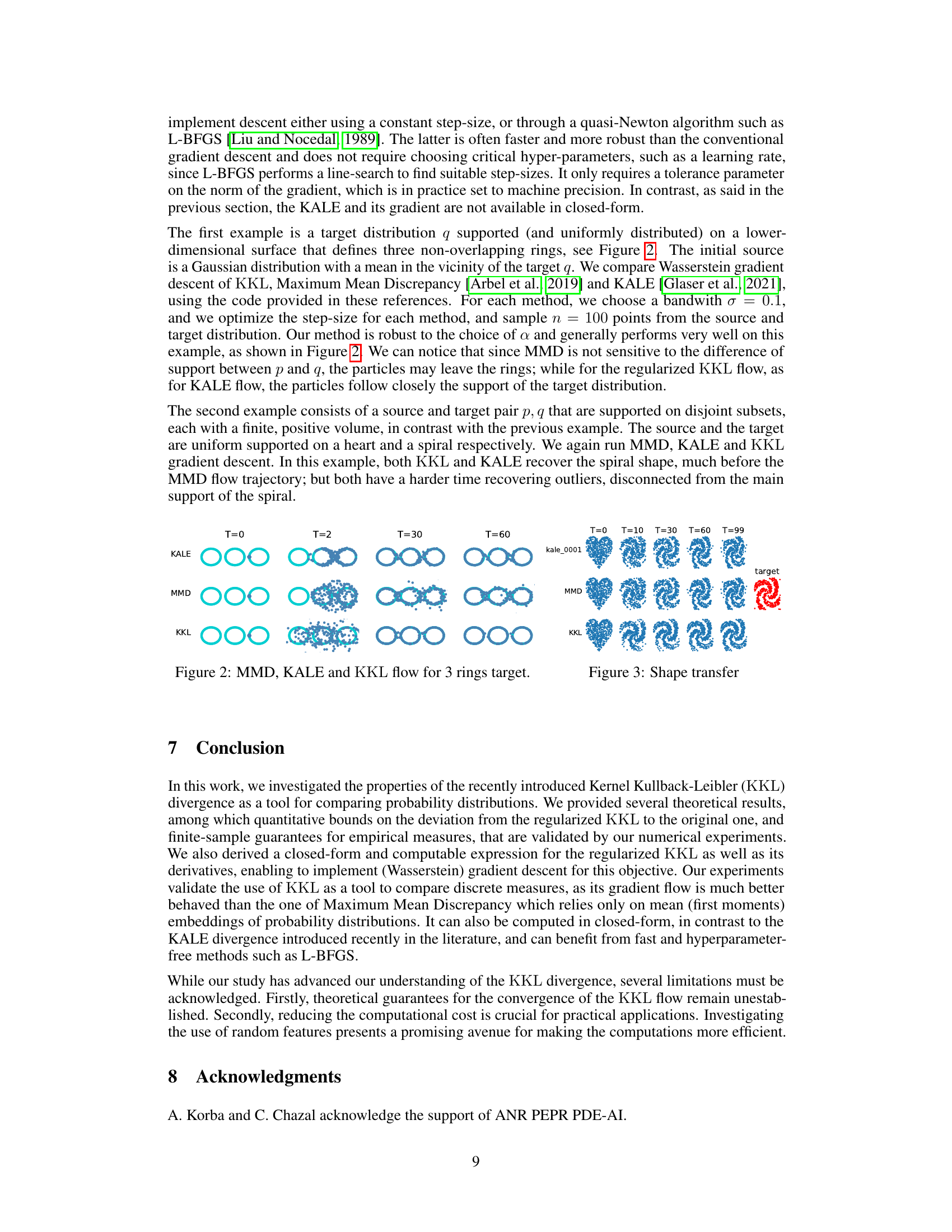
This figure compares the performance of three different methods: MMD, KALE, and KKL, in transporting a set of points (the source distribution) towards a target distribution shaped like three non-overlapping rings. The initial source distribution is a Gaussian distribution near the rings. The evolution of the distributions across different timesteps (T=0, T=2, T=30, T=60, T=99) is visualized, showing how the points are moved towards the target distribution over time using Wasserstein gradient descent.

Full paper

#