↗ OpenReview ↗ NeurIPS Homepage ↗ Chat
TL;DR#
Stochastic approximation (SA) algorithms are widely used to solve various problems under noisy conditions. While effective, using a constant step-size in SA introduces a bias, meaning the algorithm doesn’t converge exactly to the desired solution but rather oscillates around it. This bias is particularly problematic in machine learning applications and can significantly impact the accuracy of the results. This paper focuses on constant-step SA algorithms with Markovian noise (where the noise follows a Markov chain), a setting frequently encountered in real-world applications. Previous research often overlooked the dependency of noise on algorithm parameters; this study explicitly addresses this dependency.
The researchers propose a novel method to precisely quantify this bias using infinitesimal generator comparisons and semi-groups. They show that under specific conditions, the bias is of order O(α), where α is the step size. Furthermore, they demonstrate that using a time-averaged approach (Polyak-Ruppert averaging) reduces the bias to O(α²). They validate their findings through numerical simulations, showcasing that a Richardson-Romberg extrapolation technique can significantly reduce bias and enhance algorithm accuracy. This is a significant contribution as it provides a framework for understanding and controlling the bias in a common type of SA algorithm. The findings provide valuable tools for improving the performance of stochastic algorithms across a variety of applications.
Key Takeaways#
Why does it matter?#
This paper is crucial for researchers working with stochastic approximation algorithms, especially those involving constant step sizes and Markovian noise. It provides a novel framework to analyze the bias inherent in these algorithms, offering tools to quantify and mitigate this bias. This is highly relevant given the wide use of SA in machine learning and reinforcement learning, where constant step sizes are common. The findings pave the way for developing more accurate and efficient stochastic algorithms.
Visual Insights#

This figure shows sample trajectories of three different estimators of the parameter θ in a stochastic approximation algorithm with constant step size α and Markovian noise. The three estimators are: the standard iterative estimator θn, the Polyak-Ruppert average θn, and a modified Polyak-Ruppert average θn/2:n which averages only the second half of the iterations. The figure illustrates the impact of the step size α on the estimators’ convergence and bias. Smaller step sizes (α) lead to a reduced variance and bias in the Polyak-Ruppert averages.

The figure compares three different ways to estimate the parameter θ* of a stochastic approximation algorithm with Markovian noise and a constant step size α. θn represents the value of the algorithm at iteration n, θn is the Polyak-Ruppert average (time average), and θn/2:n is a modified time average that averages only the second half of the iterations. The figure illustrates how the Polyak-Ruppert averaging and the modified time average reduce the noise in the estimates. The plots show sample trajectories for different values of α, highlighting the effect of the step size on the bias and variance of the estimates.
In-depth insights#
Markovian SA Bias#
The concept of “Markovian SA Bias” refers to the systematic error or deviation observed in stochastic approximation (SA) algorithms when the underlying noise process follows a Markov chain. This bias arises because the Markov noise’s dependence on the algorithm’s current state introduces a correlation that prevents convergence to the true value. Understanding this bias is crucial for the reliable application of SA in various fields. The magnitude of this bias is directly affected by the step size parameter within the SA algorithm: smaller step sizes generally lead to smaller biases. However, excessively small step sizes might result in impractically slow convergence. Researchers often employ techniques like Polyak-Ruppert averaging to mitigate this bias, although it doesn’t eliminate it entirely. Furthermore, the specific structure of the Markov chain significantly impacts the bias’s characteristics, requiring careful consideration of the noise model in any analysis. Advanced techniques like Richardson-Romberg extrapolation are sometimes used to further reduce the bias and improve accuracy. Overall, Markovian SA bias is a nuanced challenge that demands careful attention to both theoretical analysis and practical implementation details to ensure the accuracy and effectiveness of the SA method.
Generator Comparisons#
The method of ‘Generator Comparisons’ in this context likely involves a mathematical framework to analyze stochastic approximation algorithms. It compares the infinitesimal generators of a stochastic system (the algorithm) and its deterministic counterpart (the associated ordinary differential equation, or ODE). This comparison provides a way to quantify the distance between the stochastic and deterministic dynamics. The core idea is to bound the error introduced by the stochasticity of the algorithm by relating it to the difference between the generators. This approach offers a powerful tool for analyzing the bias and convergence of stochastic approximation algorithms, particularly those with Markovian noise, as it allows for a rigorous quantification of the algorithm’s behavior relative to its deterministic limit. Smoothness conditions on the involved functions are likely assumed, to enable the application of the generator comparison technique. The resulting analysis likely offers valuable insights into the algorithm’s long-term behavior and its dependence on parameters such as step-size. A key strength is its applicability to Markovian noise, where traditional approaches might be less effective. By systematically comparing the generators, the method aims to offer tighter bounds on convergence rates and biases compared to existing methods.
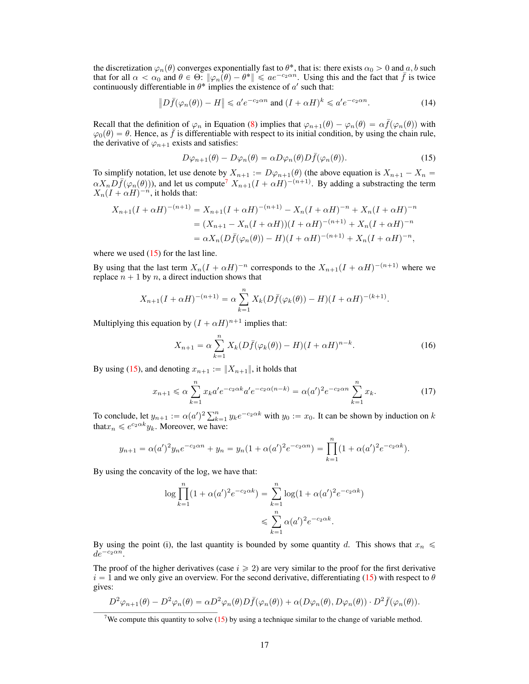
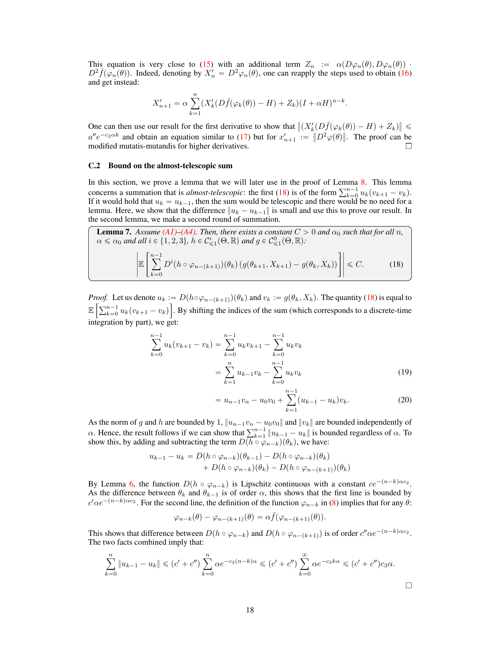
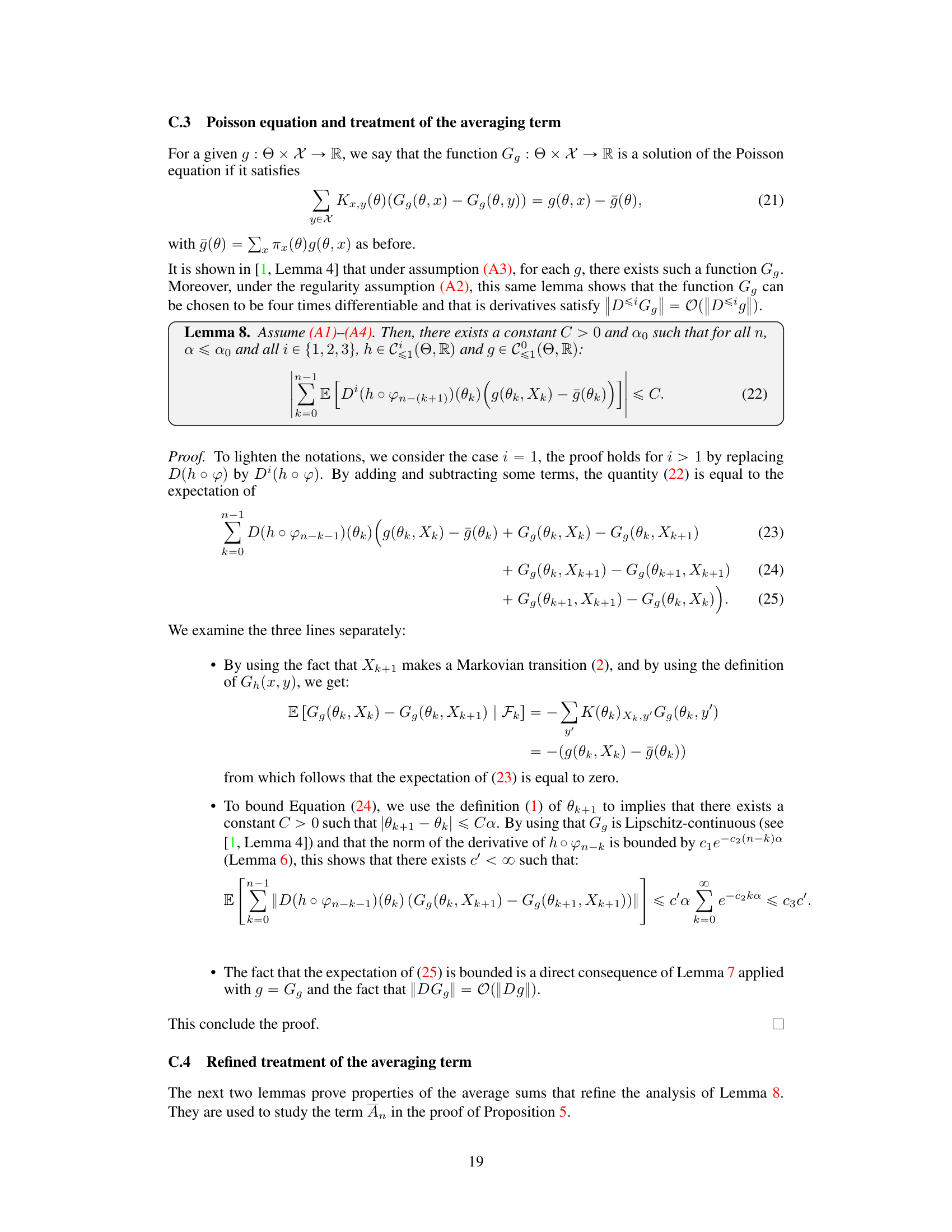
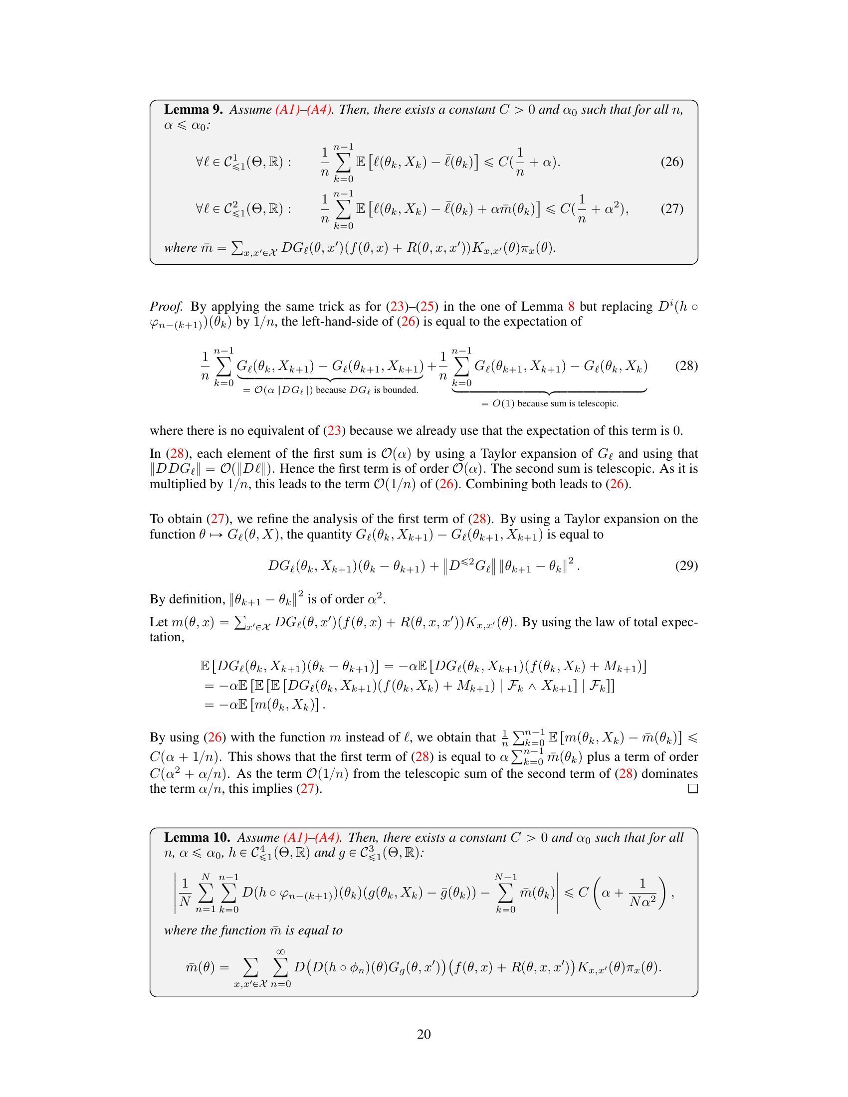
Bias Order Analysis#
A bias order analysis in a stochastic approximation algorithm investigates how the algorithm’s error, or bias, scales with respect to a step size parameter. It’s crucial to determine if the bias is vanishing (converges to zero as the step size shrinks) or persistent (remains at a certain level irrespective of step size reduction). The analysis typically involves deriving bounds on the expected difference between the algorithm’s output and the true solution. A lower bias order, such as O(α), where α is the step size, indicates a faster convergence rate to the true solution. Higher-order analysis, such as O(α²) or beyond, might involve techniques like Taylor expansion or martingale techniques to approximate the algorithm’s behavior. The results provide insights into algorithm efficiency and guide selection of optimal step sizes, balancing bias and variance for effective optimization. Understanding the bias order is essential to assess an algorithm’s performance and its applicability to diverse problem settings.
Extrapolation Methods#
Extrapolation methods, in the context of stochastic approximation, aim to improve the accuracy of estimations by leveraging information from multiple runs with varying step sizes. Richardson-Romberg extrapolation, for instance, is a powerful technique that combines estimates from different step sizes to reduce bias and achieve higher-order accuracy. This is particularly useful when dealing with constant step-size algorithms, which inherently have a bias. By strategically combining results, extrapolation methods effectively mitigate the inherent limitations of constant step-size stochastic approximations. The core idea is to extrapolate the results towards the true value by modeling the bias as a function of the step size, thus enabling a more accurate estimate of the target quantity. While extrapolation enhances accuracy, it’s important to note that the effectiveness depends heavily on the smoothness of the underlying functions and the behavior of the noise; in scenarios with highly irregular behavior, the accuracy gains might be limited. Therefore, understanding the bias structure and the noise characteristics is crucial for successful application of extrapolation methods in stochastic approximation.
Future Work#
The paper’s absence of a dedicated ‘Future Work’ section presents an opportunity to thoughtfully consider potential research extensions. One key area would be relaxing the assumption of a compact state space for the parameter θ. This is a significant restriction, limiting the applicability of the results. Exploring methods to handle unbounded parameter spaces, perhaps through the use of large deviation techniques, would greatly expand the scope. Further investigation into the impact of non-differentiable functions f is also warranted. The current analysis relies heavily on differentiability; investigating alternative approaches for non-smooth functions would be valuable, potentially employing techniques from non-smooth optimization. Finally, a detailed empirical study comparing the proposed method to existing state-of-the-art algorithms, especially in high-dimensional settings, is essential to validate its practical benefits. Such a comparison should consider the trade-offs between bias reduction and computational complexity. Addressing these areas would significantly enhance the paper’s contribution and impact.
More visual insights#
More on figures
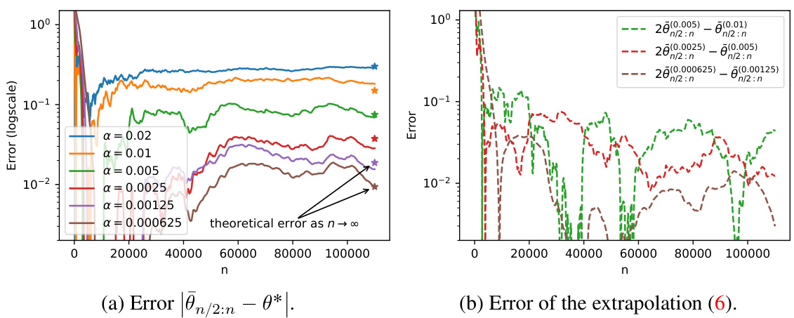
The figure shows sample trajectories of three different estimators for the parameter θ in a stochastic approximation algorithm with Markovian noise and constant step size α. The estimators are: θn (the standard iterative estimator), θn (the Polyak-Ruppert average), and θn/2:n (a modified Polyak-Ruppert average starting from the middle of the trajectory). The plots illustrate the convergence behavior of these estimators for different values of α, demonstrating how the bias and variance of the estimates change with the step size. In particular, it shows how the Polyak-Ruppert average significantly reduces the variance and improves the estimate’s closeness to the true value, even more so when starting the average from halfway through the trajectory.
This figure compares the performance of three different estimators for the parameter θ in a stochastic approximation algorithm with Markovian noise and constant step size α. The three estimators are: 1. θn: The raw, un-averaged estimate at iteration n. 2. θn: The Polyak-Ruppert average of θn over all iterations up to n. 3. θn/2:n: The Polyak-Ruppert average of θn from iteration n/2 to n. The figure shows sample trajectories for various values of α (step sizes). It demonstrates that Polyak-Ruppert averaging significantly reduces the noise in the estimate compared to the raw estimate (especially for small α). Averaging only over the latter half of the iterations (θn/2:n) also exhibits a better convergence rate than averaging over all iterations (θn).

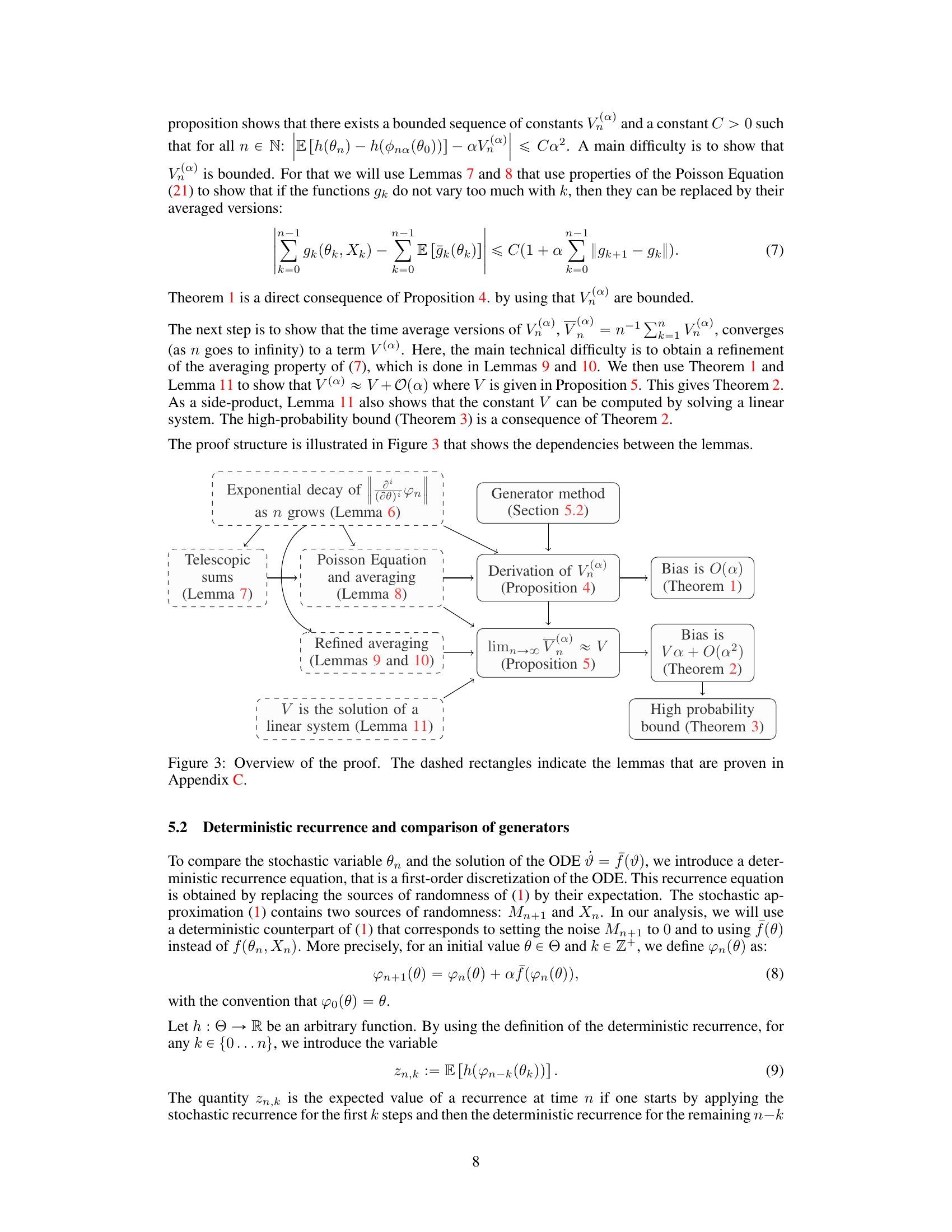
This figure illustrates the comparison between the stochastic recurrence and its deterministic counterpart. The left panel shows the trajectories of θn and φn(θ0) for the same source of randomness. The right panel shows the effect of changing the value of k in φn−k(θk). For n > k, it represents the stochastic recurrence applied to the first k steps and then the deterministic recurrence for the remaining steps (n−k). For n < k, it represents only the deterministic recurrence. The figure is used to illustrate the methodology of the proof in Section 5.2.

This figure compares the behavior of three different estimators of the root of the ODE (θ*, which is 1 in the example) as a function of the step size α. The first estimator (θn) is the direct output of the stochastic approximation algorithm, while the other two (θn and θn/2:n) use Polyak-Ruppert averaging to reduce the variance. The plots show sample trajectories for various values of α, highlighting how the averaging techniques improve the accuracy of the estimation. The plot shows that the Polyak-Ruppert averaging significantly reduces the variance, bringing the estimate closer to the true value (θ* = 1). This improvement is more pronounced for smaller values of α.
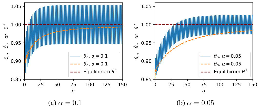
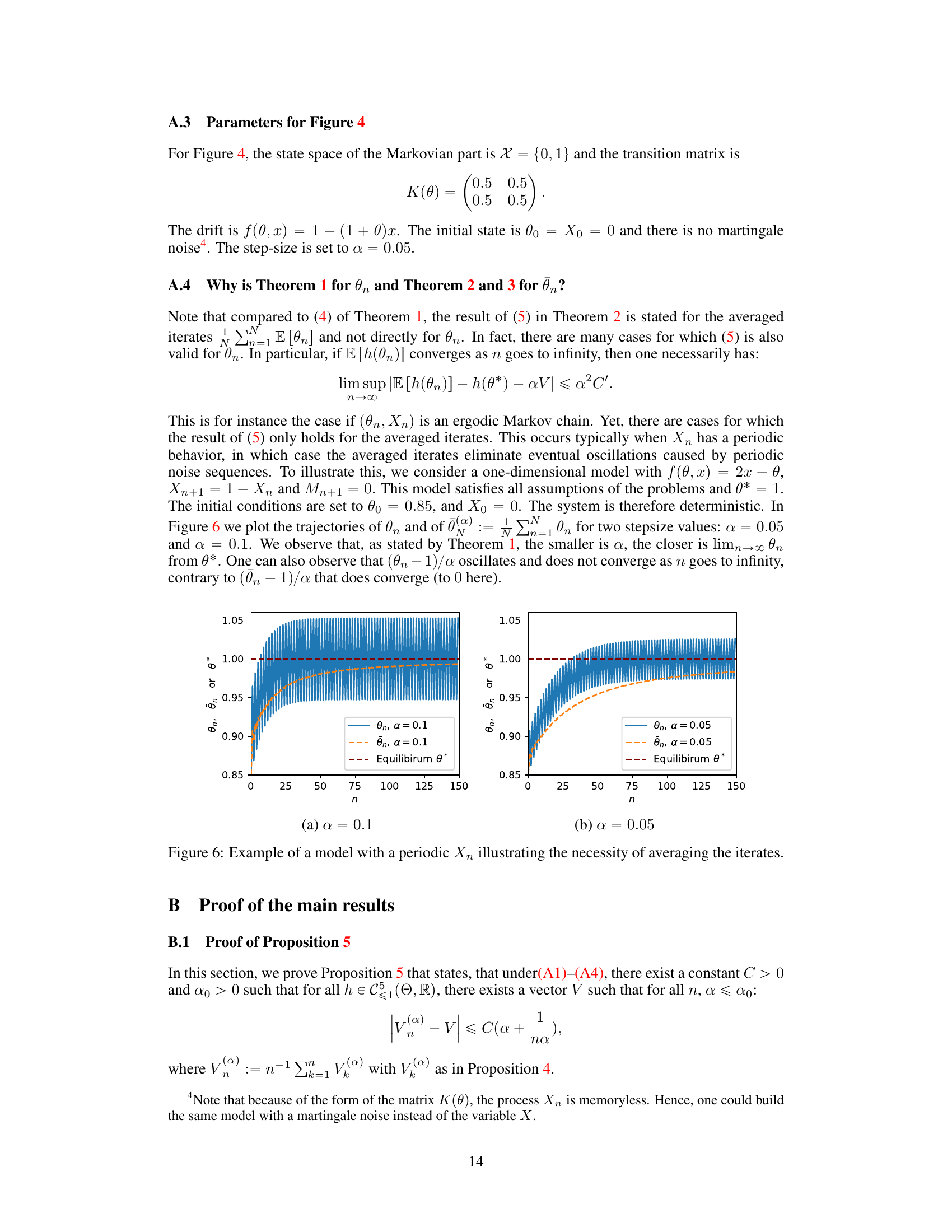
This figure shows the necessity of averaging the iterates when the Markov chain Xn is periodic. Two plots are presented, illustrating the behavior of the iterates θn and their averages θn for different step sizes (α = 0.1 and α = 0.05). While the averaged iterates θn converge smoothly toward the equilibrium θ*, the non-averaged iterates θn exhibit oscillations due to the periodic nature of Xn, highlighting the importance of averaging to obtain stable results.
More on tables

This figure compares the behavior of three estimators of the root θ* of the ODE in a synthetic example. θn represents the direct output of the constant-step stochastic approximation algorithm. θn is the Polyak-Ruppert average of θn. θn/2:n is a modification of the Polyak-Ruppert average starting from the middle of the trajectory. The figure shows sample trajectories for different values of the step size α. The purpose is to illustrate that the Polyak-Ruppert average and its modification significantly reduce the variance and approach the true value faster than the direct estimator θn, especially when α is small.

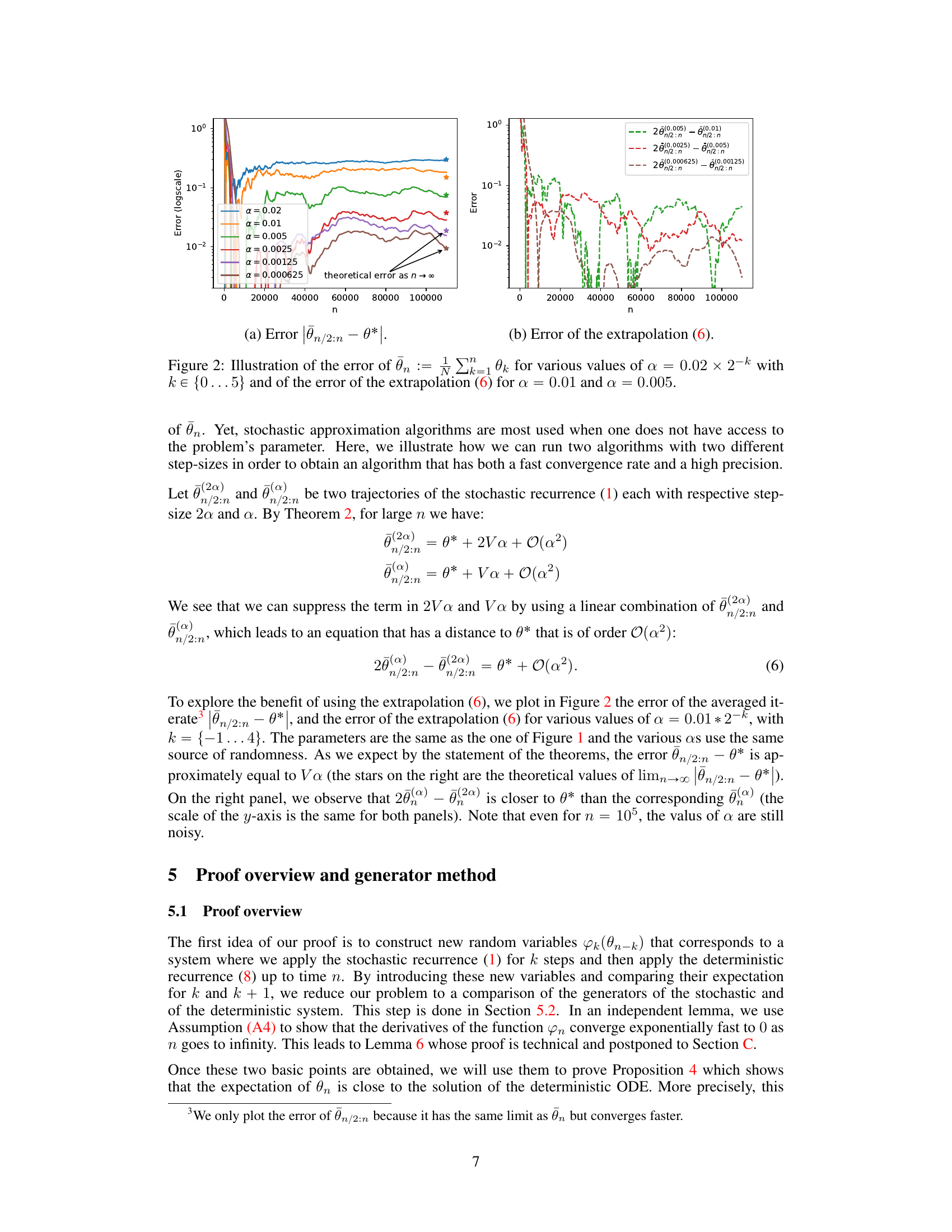
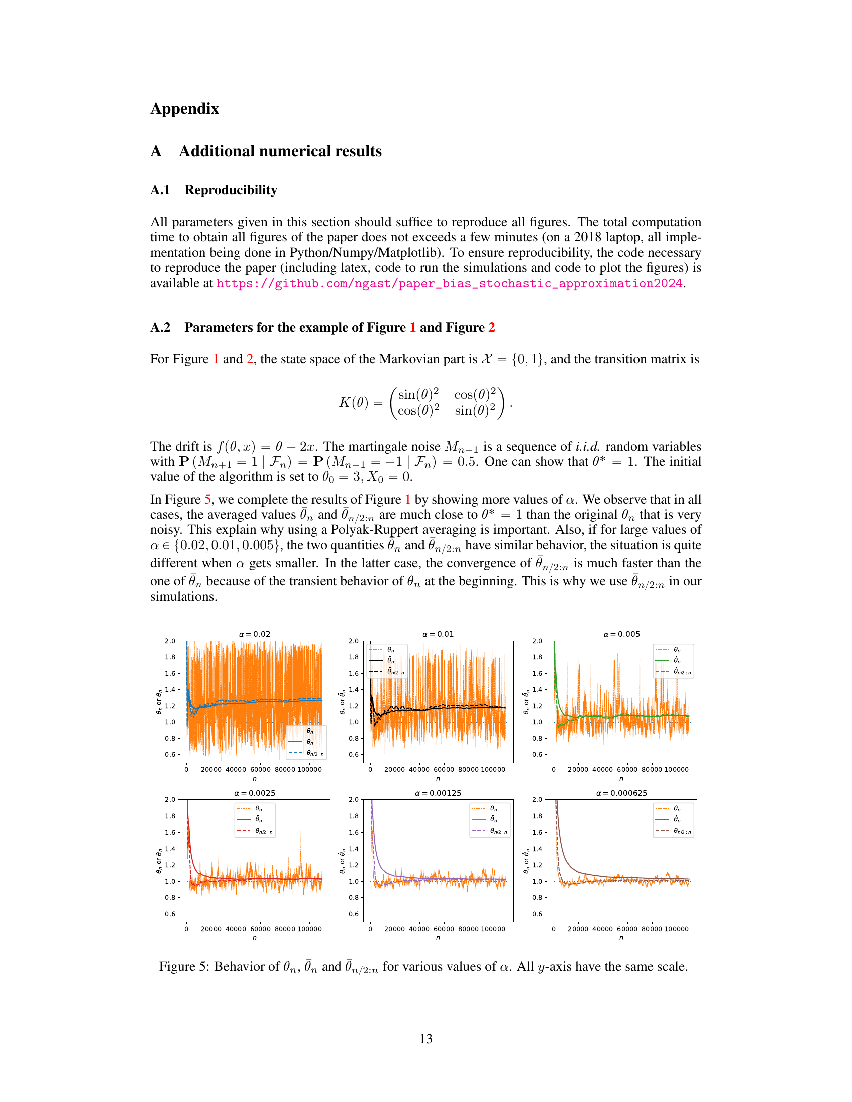
This figure shows sample trajectories of three different estimators of the parameter θ* in a stochastic approximation algorithm: θn, the standard estimator; θn, the Polyak-Ruppert average; and θn/2:n, a modified Polyak-Ruppert average that averages only the second half of the trajectory. Different plots show the results for different values of the step size α, ranging from 0.02 to 0.000625. The figure illustrates how the Polyak-Ruppert averages significantly reduce the noise and converge closer to the true parameter compared to the standard estimator. Also it shows that using only the second half of the trajectory further improves convergence for small step sizes.

This figure shows the behavior of three different estimators of the solution of a stochastic approximation problem with Markovian noise. The three estimators are: the original stochastic approximation algorithm (θn), the Polyak-Ruppert average (θn), and a truncated Polyak-Ruppert average (θn/2:n). The figure illustrates how the bias and variance of these estimators change as the step-size α decreases. The x-axis represents the iteration number, and the y-axis represents the value of the estimators. The different colors correspond to different step-size values.
Full paper#

