↗ OpenReview ↗ NeurIPS Homepage ↗ Chat
TL;DR#
Training large language models (LLMs) is computationally expensive, and finding optimal training strategies is critical. A key metric in optimizing this process is Gradient Noise Scale (GNS), which quantifies the uncertainty in the gradient calculations. Existing methods for calculating GNS are often computationally expensive and noisy.
This research presents a novel method for efficiently and accurately estimating GNS in LLMs. By focusing on normalization layers and integrating per-example gradient norm calculations directly into the LayerNorm backward pass, this method avoids significant computational overhead. This technique not only improves GNS estimations but also enables the development of more efficient training schedules, leading to substantial time savings in training.
Key Takeaways#
Why does it matter?#
This paper is crucial for researchers working with large language models due to its focus on efficiently estimating gradient noise scale (GNS), a key factor in optimizing training. The proposed method offers significant speedups, making it highly relevant for researchers facing computational constraints. It also opens new avenues for research by demonstrating the strong correlation between layer-specific GNS and overall model GNS, potentially leading to improved training strategies.
Visual Insights#

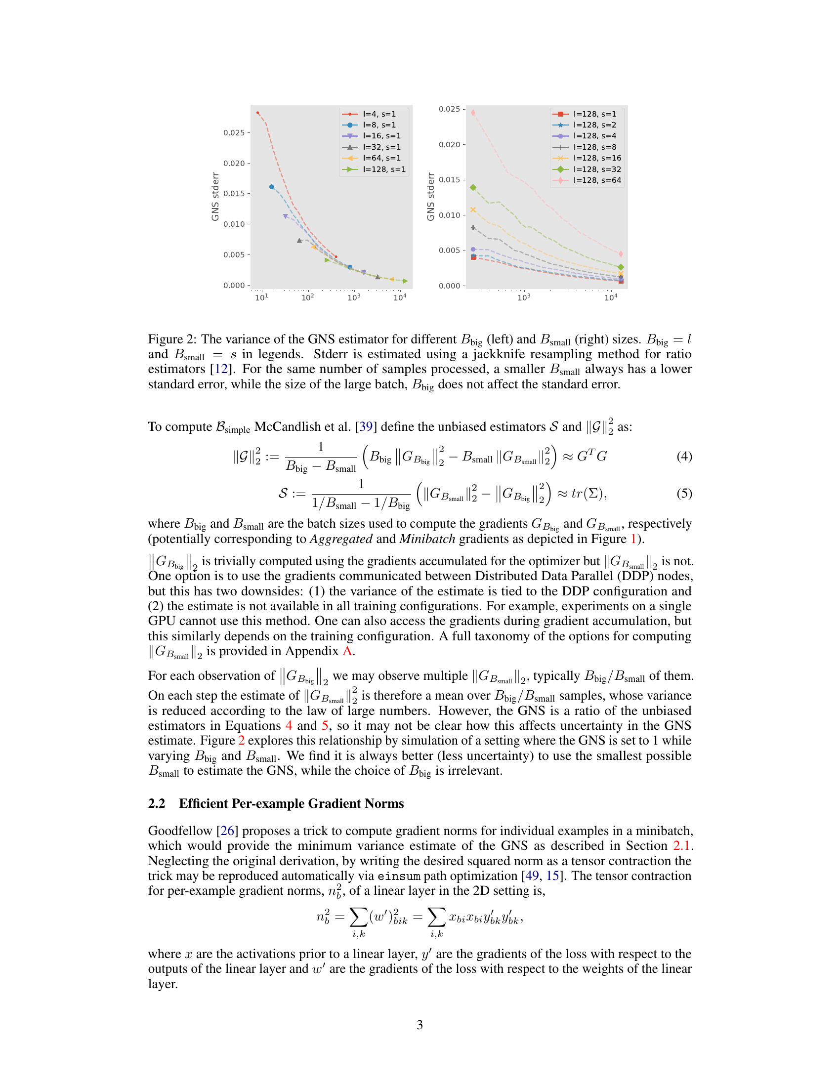
This figure shows the variance of the Gradient Noise Scale (GNS) estimator as a function of the batch sizes used for computation (Bbig and Bsmall). The left panel demonstrates that the standard error of the GNS estimator decreases as Bsmall decreases, while it is unaffected by changes in Bbig. The right panel shows the same trend for different values of Bbig.
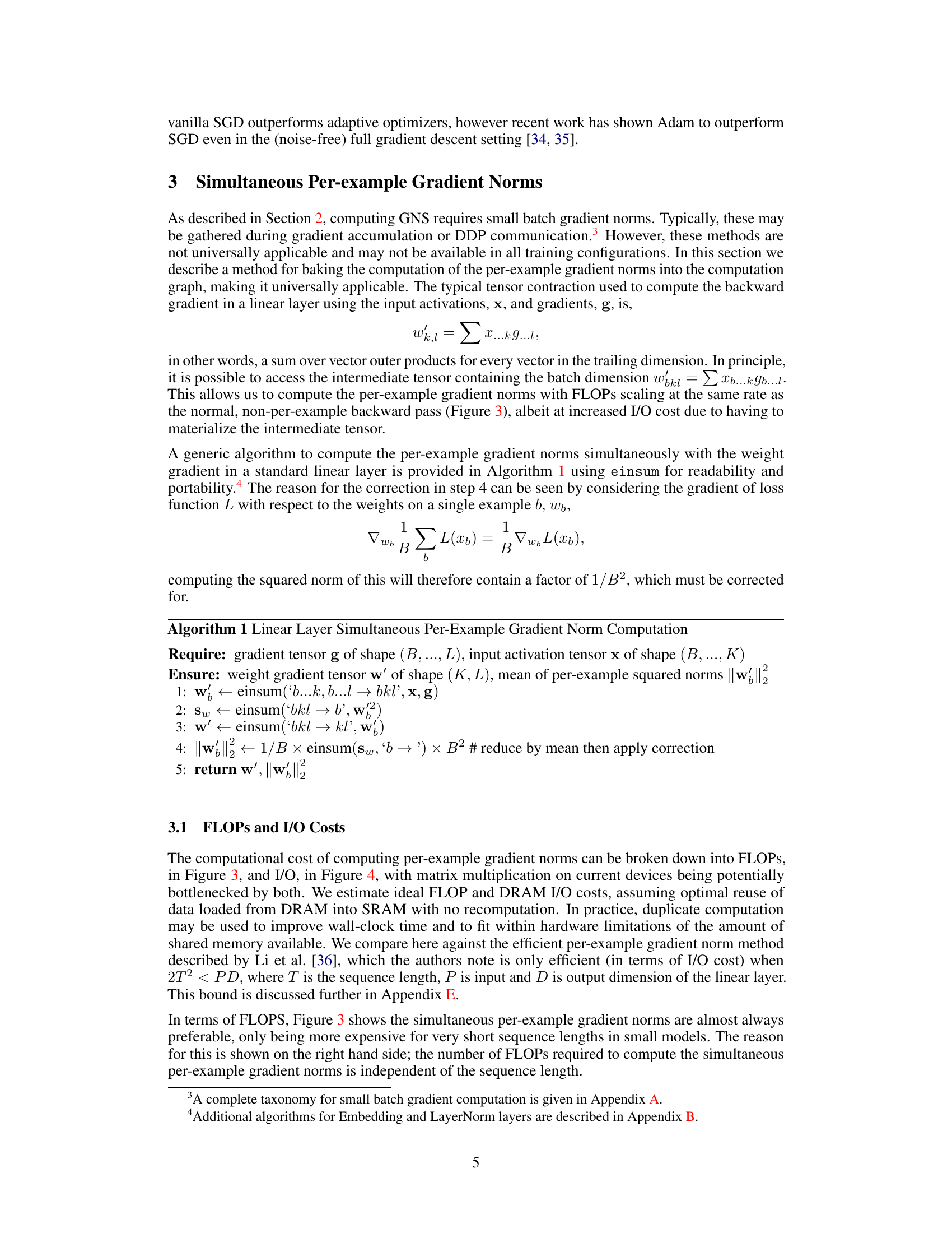
This table shows the FLOP counts for computing weight gradients and gradient norms using the simultaneous method proposed in the paper and the method by Li et al. [36]. It breaks down the FLOP costs based on the dimensions of the input and output tensors and the sequence length, highlighting the computational efficiency of the proposed simultaneous approach.
In-depth insights#
GNS in Transformers#
The study explores Gradient Noise Scale (GNS) within the context of transformer models, a crucial metric for optimizing training efficiency. The core finding highlights the strong correlation between the GNS of normalization layers and the overall GNS of the entire transformer model. This suggests that monitoring only normalization layers can effectively predict and guide the GNS, thus simplifying the GNS estimation process. The research introduces a custom kernel for efficiently computing per-example gradient norms during LayerNorm’s backward pass, eliminating throughput overhead. This allows practical application of GNS tracking for batch size scheduling, leading to demonstrable improvements in training speed, as evidenced by an 18% reduction in training time for a Chinchilla-optimal language model. The work contributes valuable insights into the GNS behavior in Transformers, offering effective methods for its measurement and utilization in improving training optimization.
Efficient GNS Metric#
An efficient Gradient Noise Scale (GNS) metric is crucial for effective large-scale model training. The paper focuses on optimizing GNS computation, emphasizing the importance of per-example gradient norms for minimizing variance. A key contribution is the development of a method to compute these norms concurrently with the parameter gradient calculation, resulting in zero throughput overhead. This approach contrasts with existing methods that introduce significant computational costs or rely on approximations. The authors demonstrate that GNS for normalization layers correlates strongly with the overall GNS of the model, enabling a computationally inexpensive approximation. This allows for efficient batch size scheduling, improving training time. The proposed method’s efficiency is experimentally validated, showcasing improved performance compared to alternative GNS estimation techniques. Furthermore, a custom kernel significantly accelerates LayerNorm backward pass, enabling zero computational overhead during GNS computation. While primarily focused on Transformers, the underlying principles are applicable to other neural network architectures with suitable adaptations.
Batch Size Schedule#
The research explores batch size scheduling as a method to optimize training efficiency in large language models. The core idea revolves around dynamically adjusting the batch size during training, rather than using a fixed size throughout. This approach is motivated by the observation that the optimal batch size often changes during different training phases. The study employs a custom kernel that simultaneously calculates the per-example gradient norms and LayerNorm backward passes, eliminating computational overhead. By using gradient noise scale (GNS) as a guide, this scheduling method aims to reduce training time. A key finding is the strong correlation between the GNS of LayerNorm layers and the overall GNS, allowing efficient GNS tracking solely on normalization layers. The effectiveness of this approach is demonstrated through a practical case study, achieving an 18% reduction in training time on a Chinchilla-optimal language model. This highlights the potential of GNS-guided batch size scheduling as a valuable technique for optimizing training efficiency in large-scale models.
LayerNorm’s Role#
The research paper highlights the pivotal role of Layer Normalization (LayerNorm) layers in predicting the gradient noise scale (GNS) of transformer models. LayerNorm layers exhibit a strong correlation with the overall GNS, simplifying GNS estimation by focusing computation on these layers alone. This is a significant finding because calculating GNS usually requires computationally expensive per-example gradient norm computations across all layers. The custom kernel developed to compute these norms during the LayerNorm backward pass demonstrates zero throughput overhead, leading to significant efficiency gains. This efficiency allows for practical batch size scheduling and GNS tracking during training, ultimately improving training speed. The research strongly suggests that LayerNorm’s internal dynamics are highly informative about the overall model’s training behavior and noise characteristics. Therefore, understanding and leveraging LayerNorm’s GNS is crucial for optimizing the training process of large transformer models. The simplicity and efficiency of focusing on LayerNorm, as opposed to the whole model, holds immense potential for streamlining training large neural networks.
Future Research#
Future research directions stemming from this work could explore extending the per-example gradient norm computation to a wider array of neural network architectures beyond Transformers. RNNs and CNNs, for instance, could benefit from efficient per-example gradient norm calculations to improve GNS estimation and batch size scheduling. Further investigation into the theoretical underpinnings of the GNS, especially concerning its behavior with non-diagonal Hessians, is warranted. Developing a more comprehensive understanding of the interplay between GNS, architectural choices (e.g., wider vs. narrower networks), and dataset characteristics would offer valuable insights into optimization strategies for large-scale models. Finally, applying the efficient GNS tracking techniques to a broader range of tasks and model sizes would allow us to ascertain the universality and effectiveness of these methods. A strong emphasis on investigating the practical implications and limitations of GNS-guided batch size scheduling in production environments is crucial. This would help validate the potential gains realized in training time reduction in practical, large-scale scenarios.
More visual insights#
More on figures
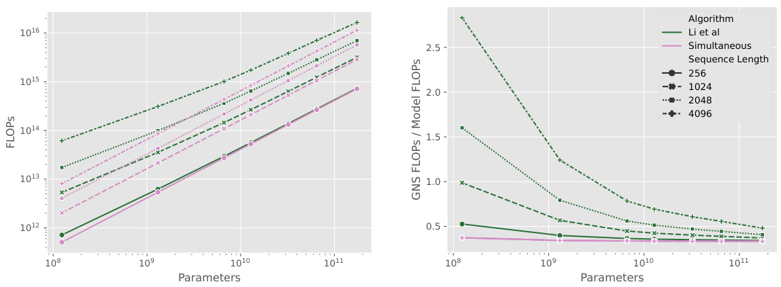
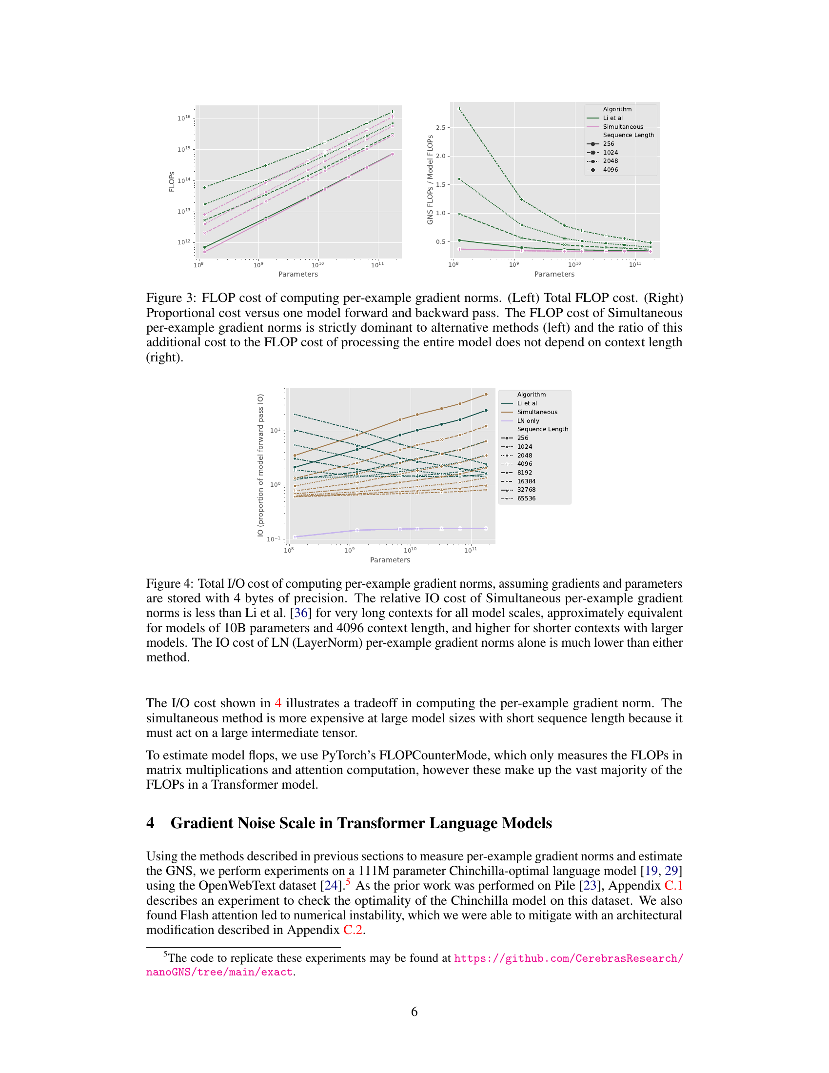
This figure compares the FLOP cost of three methods for computing per-example gradient norms against the total FLOP cost of a forward and backward pass of a neural network model. The left panel shows the total FLOP cost for each method, while the right panel shows the ratio of the per-example gradient norm FLOP cost to the total model FLOP cost. The ‘Simultaneous’ method consistently outperforms the other methods in terms of FLOPs, especially for longer sequences. The ratio of the additional FLOP cost to the total model FLOP cost remains relatively constant across different sequence lengths for the Simultaneous method.

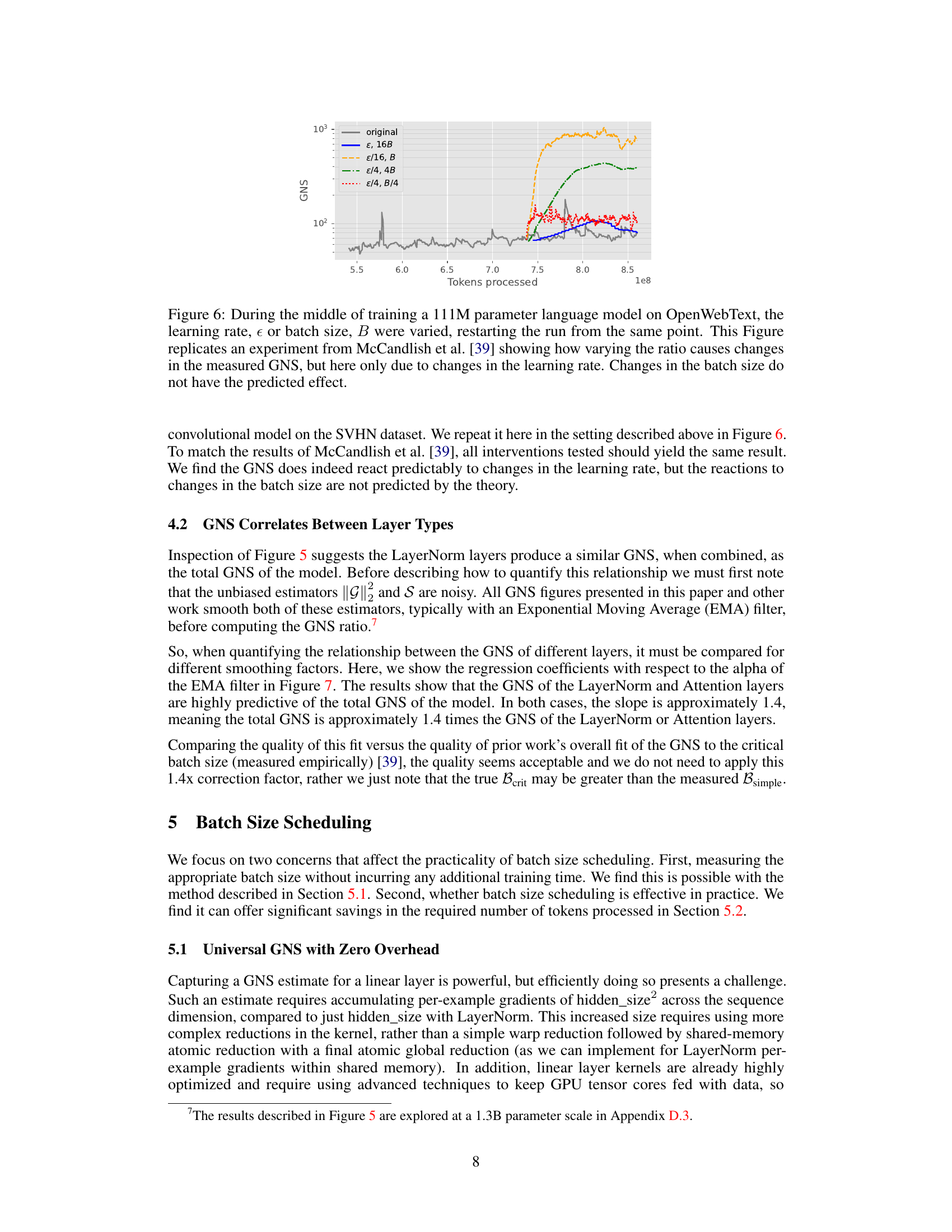
This figure compares the I/O cost of three different methods for computing per-example gradient norms: the method proposed in the paper (Simultaneous), the method by Li et al. [36], and a method that only considers LayerNorm layers (LN only). The results show that the Simultaneous method is more efficient for longer sequences and larger models. The LN only method is significantly more efficient than the others, suggesting that focusing on LayerNorm layers is sufficient for accurate GNS estimation. The I/O cost is shown as a proportion of the model’s forward pass I/O cost.

This figure shows the GNS (Gradient Noise Scale) phase plot. It visualizes the relationship between two estimators of GNS (||G||² and S) and the overall GNS, across different layers of a neural network during training. The left plots show the component estimators for linear/embedding layers and LayerNorm layers separately. The right plots show the overall GNS trends for each layer type and a combined GNS, providing a visual representation of how the different components contribute to the overall gradient noise scale over the training process.
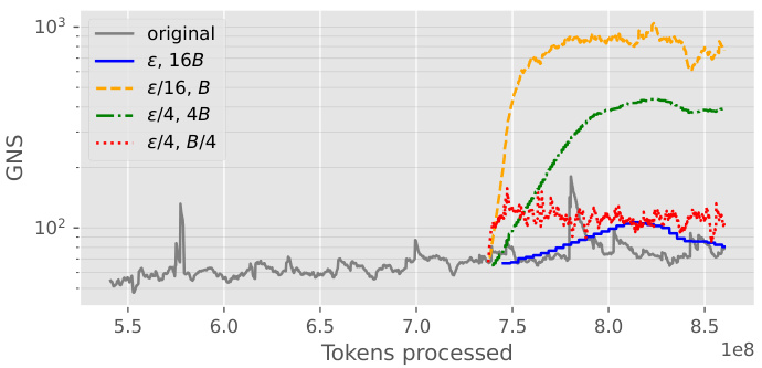
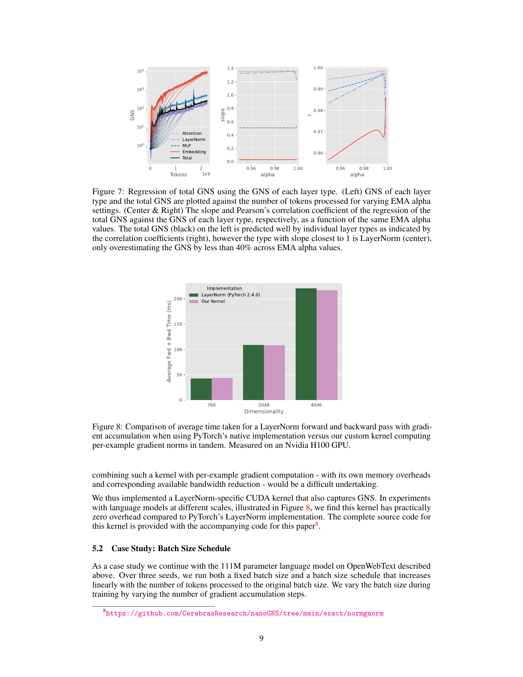
This figure replicates an experiment from a previous work which shows how changing the ratio of batch size to learning rate affects the Gradient Noise Scale (GNS). The authors of this paper varied the learning rate and batch size independently, keeping their ratio constant, and found that only changes in the learning rate affected the GNS, while changes in the batch size did not.
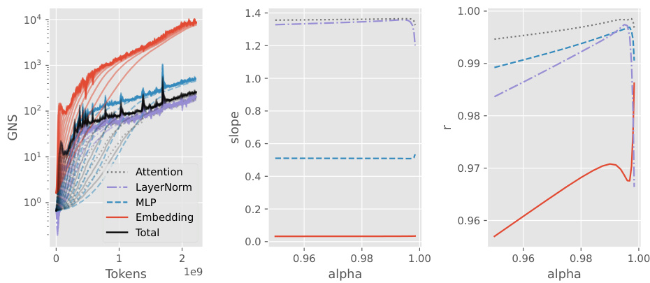
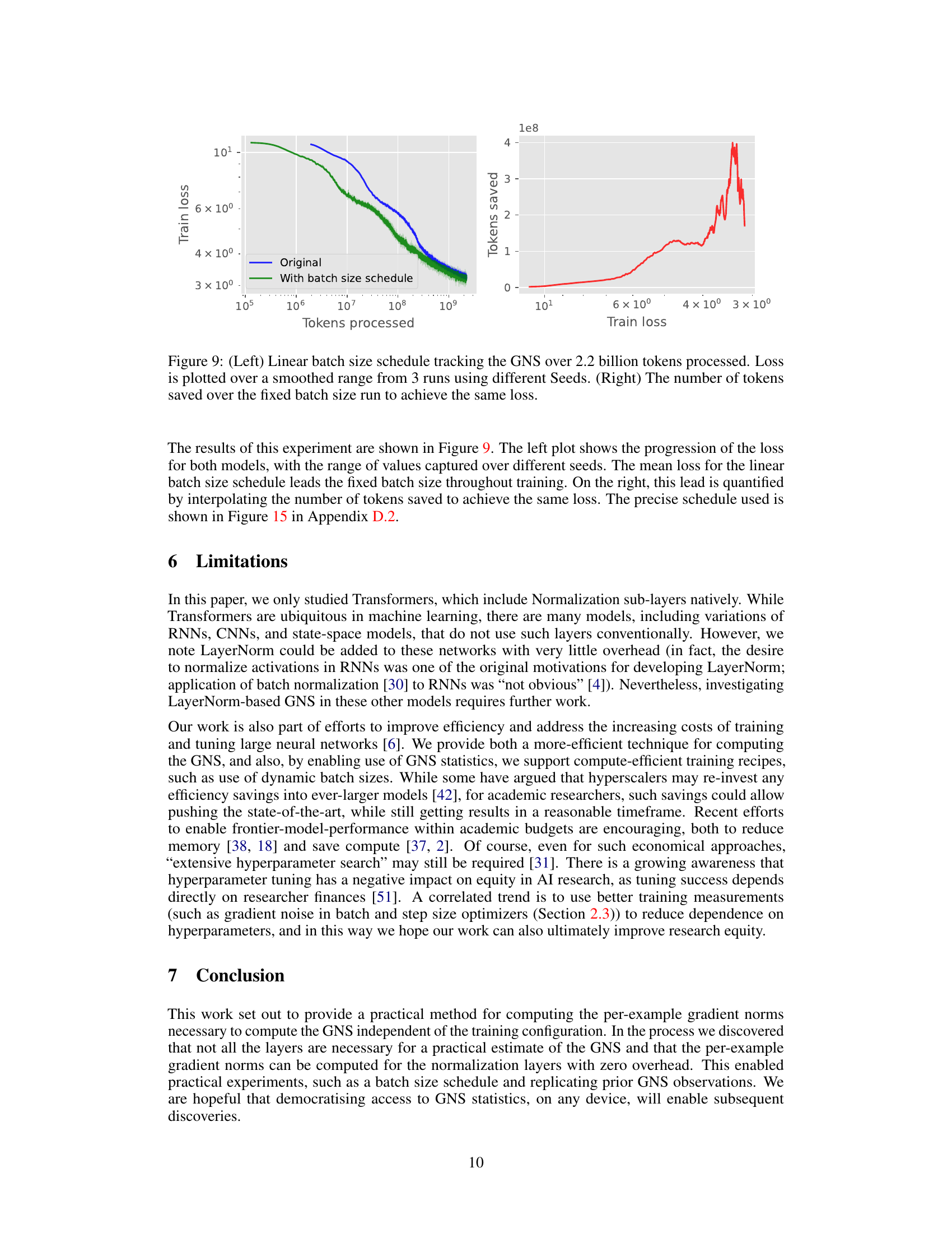
This figure shows the relationship between the total gradient noise scale (GNS) of a transformer model and the GNS of individual layer types (Attention, LayerNorm, MLP, Embedding). The left panel plots the GNS for each layer type and the total GNS against the number of tokens processed, for different values of EMA alpha (a smoothing parameter). The center and right panels show the slope and Pearson correlation coefficient, respectively, of the regression of total GNS against each layer type’s GNS, as a function of EMA alpha. The results indicate that the total GNS is strongly correlated with the GNS of individual layer types, especially LayerNorm, suggesting that monitoring LayerNorm’s GNS can provide a good estimate of the overall GNS.

This figure compares the performance of PyTorch’s built-in LayerNorm implementation against a custom kernel developed by the authors. The custom kernel is designed to simultaneously compute per-example gradient norms alongside the standard forward and backward passes of LayerNorm. The comparison is performed across varying dimensionalities (768, 2048, and 4096), showing the average time taken for both implementations. The results demonstrate that the custom kernel achieves comparable or better performance than PyTorch’s implementation, especially at higher dimensionalities. This highlights the efficiency of the proposed approach, which enables gradient noise scale (GNS) estimation with near-zero overhead.
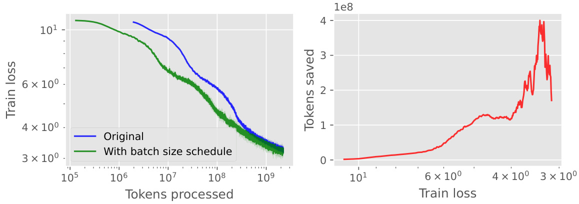
This figure shows the results of an experiment comparing a fixed batch size training schedule to one where the batch size increases linearly with the number of tokens processed. The left plot shows the training loss for both schedules over the course of training. The right plot shows the number of tokens saved by using the linear batch size schedule compared to the fixed batch size schedule, to achieve the same training loss. The results demonstrate the effectiveness of the linear batch size schedule in reducing training time.
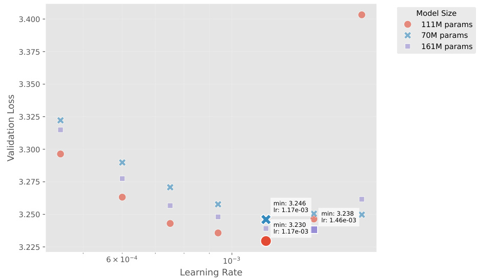
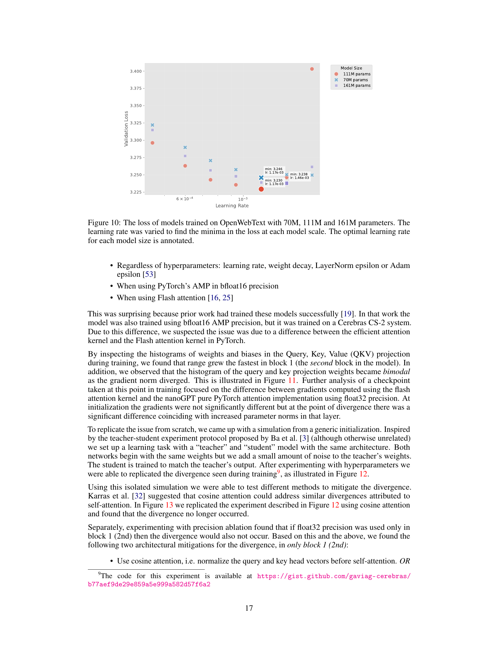
This figure shows the validation loss of three different-sized language models (70M, 111M, and 161M parameters) trained on the OpenWebText dataset. The x-axis represents the learning rate used during training, and the y-axis represents the validation loss achieved. Each model size has multiple data points, each representing a different learning rate tested. The optimal learning rate for each model size that resulted in the lowest validation loss is annotated on the plot. The goal was to determine the optimal learning rate for each model size while maintaining a constant total number of FLOPs.
This figure shows the relationship between the different components of the gradient noise scale (GNS) and the overall GNS over the course of training a language model. The left side shows the individual components (||G||² and S) for Linear/Embedding layers and LayerNorm layers separately. The right side shows the overall GNS calculated from these components. This visualization helps to understand how the different layer types contribute to the overall GNS and how these components change during training.
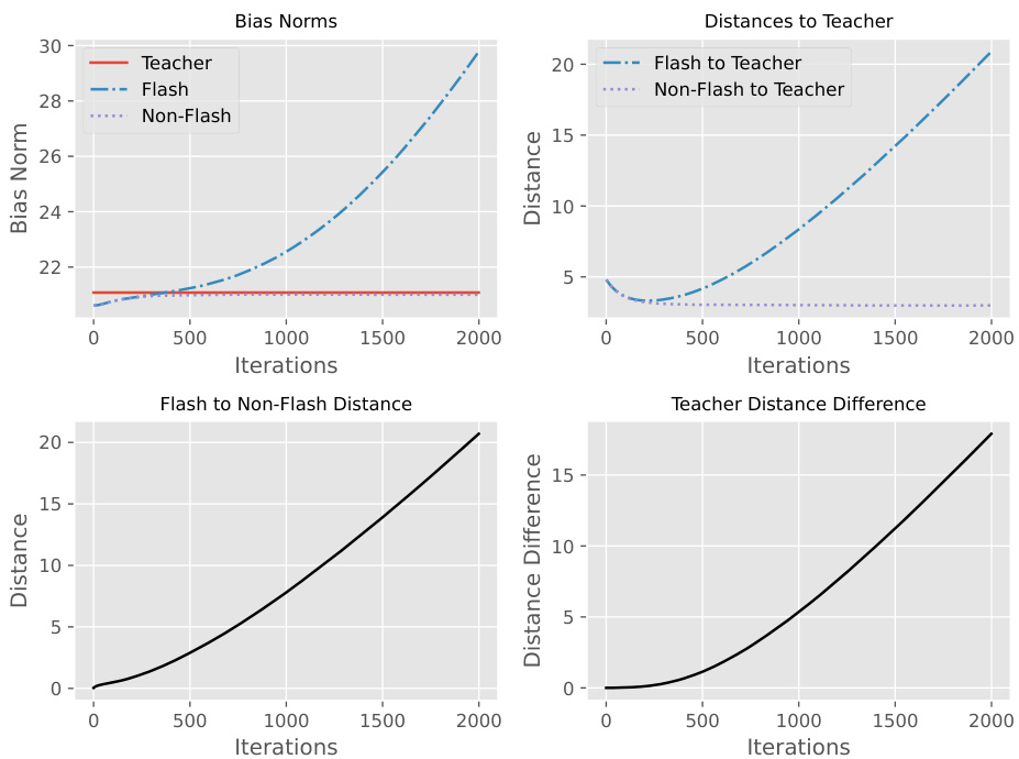
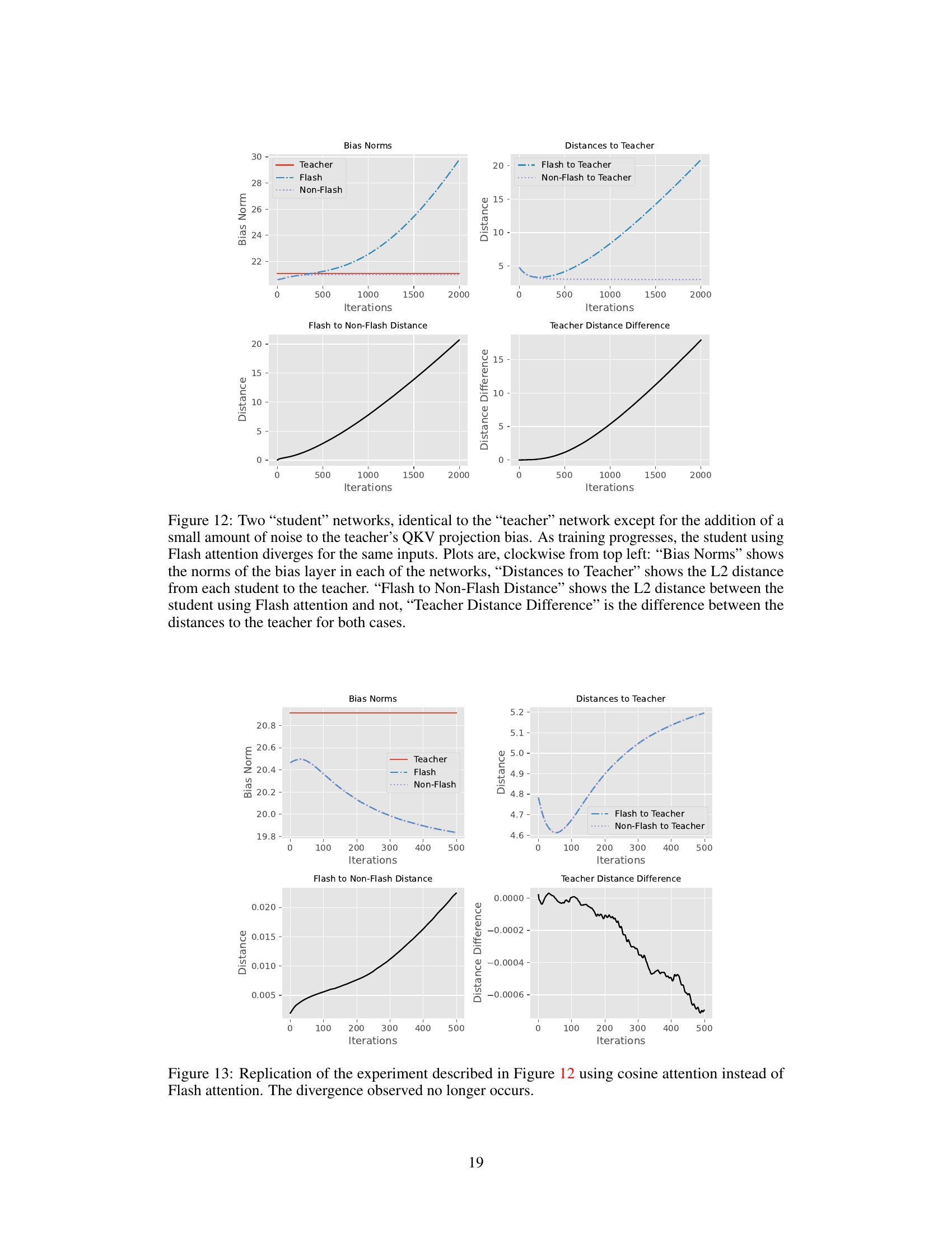
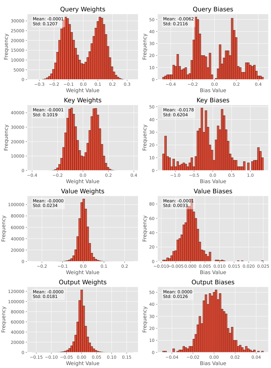
This figure shows the results of an experiment comparing two student networks trained with and without Flash Attention. Both networks start with similar weights but the teacher network has additional noise added to its weights. The plot shows that the network using Flash Attention diverges from the teacher network as training progresses, while the network without Flash Attention remains close. The different plots illustrate several metrics like bias norms, distances to the teacher, and the difference in distances between the two student networks.
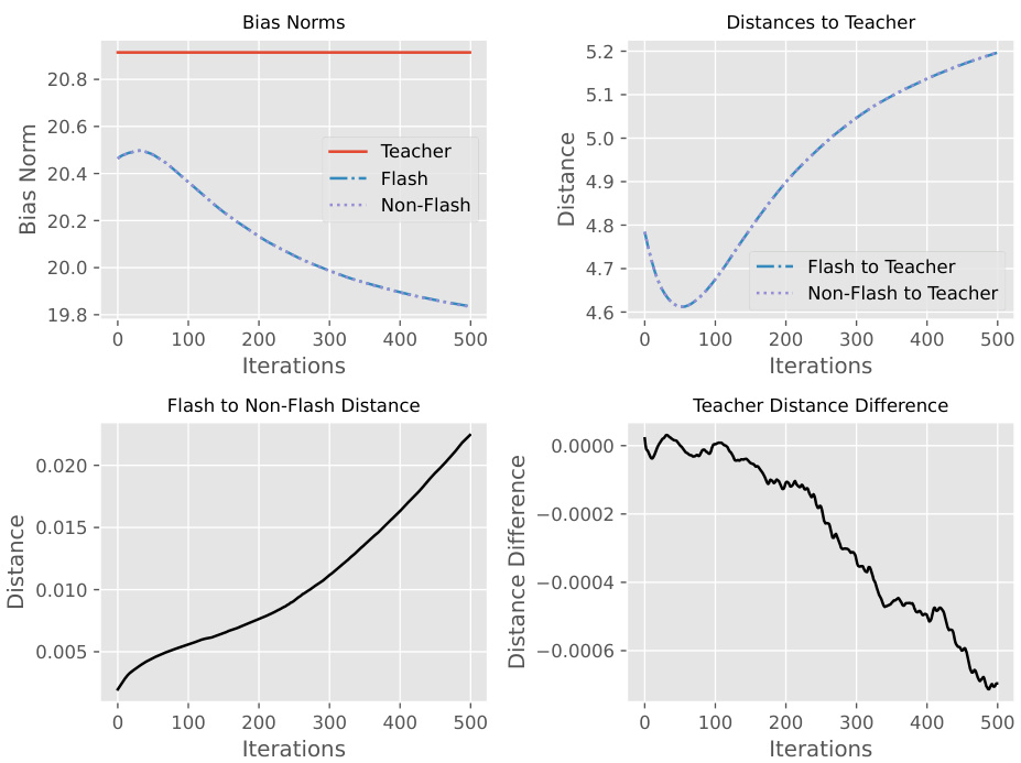
This figure shows the results of an experiment designed to simulate the divergence observed when using Flash Attention. Two networks, a teacher and a student, are trained. The student network is identical to the teacher except for a small amount of added noise to the teacher’s QKV projection bias. The plots show how the bias norms, distances to the teacher, distances between the networks (student models using Flash Attention and a control network without it), and the difference in distances to the teacher between the two networks change over training iterations. The results show that, in this simulated scenario, the student using Flash Attention diverges.
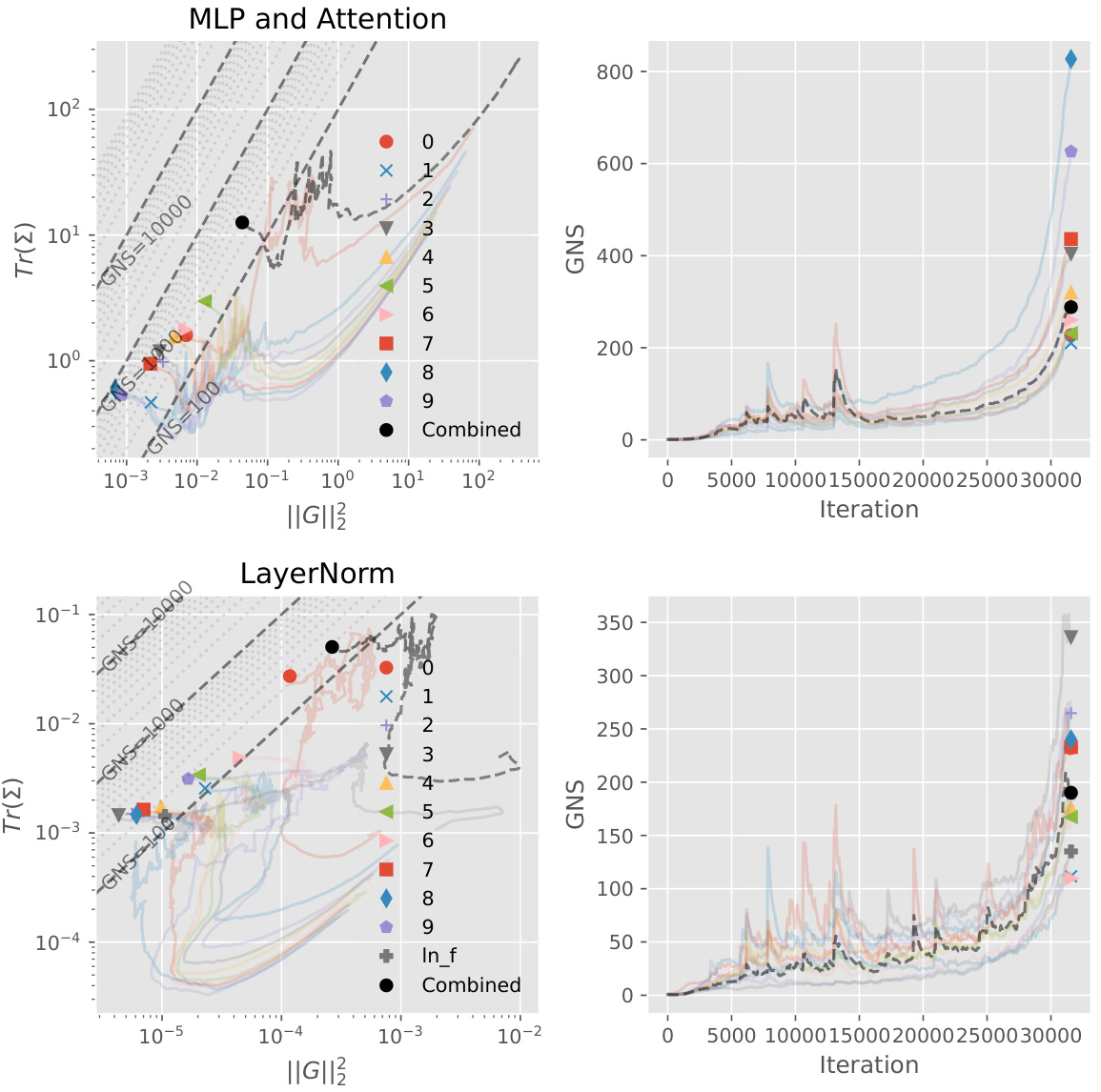
This figure visualizes the relationship between the gradient noise scale (GNS) and its component estimators (||G||2 and S) over the course of training a transformer model. It shows the GNS and its components for both linear/embedding layers and LayerNorm layers separately. The plots show that the GNS of LayerNorm layers strongly correlates with the total GNS, implying the efficiency of focusing only on the LayerNorm layers for practical GNS tracking. The ‘combined’ trace (black) shows that LayerNorm and the other layers’ GNS estimates (colored traces) trend similarly during training.

This figure shows the results of an experiment comparing a fixed batch size training schedule with a linear batch size schedule that increases linearly with the number of tokens processed. The left plot shows the training loss for both schedules, smoothed over three runs with different random seeds. The right plot shows the number of tokens saved by using the linear batch size schedule compared to the fixed batch size schedule to achieve the same loss.
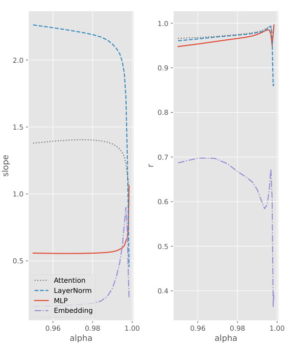
This figure shows the relationship between the total Gradient Noise Scale (GNS) of a transformer model and the GNS of individual layer types (Attention, LayerNorm, MLP, Embedding). The left panel plots the GNS values against the number of tokens processed for various EMA smoothing factors (alpha). The central and right panels show the regression slope and Pearson correlation coefficient between the total GNS and each individual layer type’s GNS as a function of the EMA alpha. The results indicate a strong correlation between the total GNS and the GNS of the LayerNorm layers, with the LayerNorm GNS being a particularly good predictor of the overall GNS.
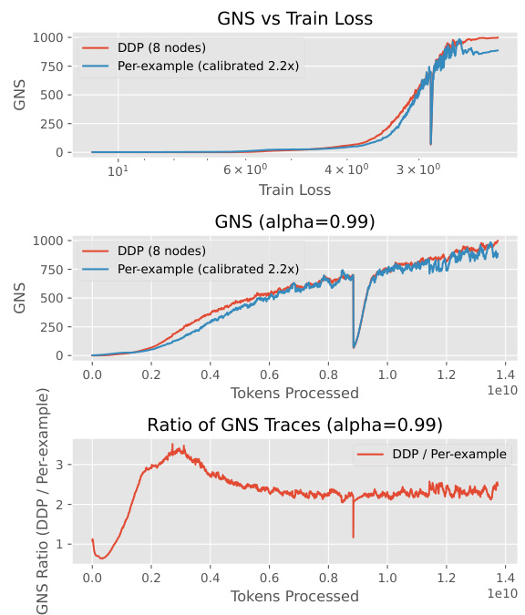
This figure compares the gradient noise scale (GNS) estimation methods for a larger 1.3B parameter GPT model trained on OpenWebText dataset using 8 H100 GPUs. The left panel shows per-example gradient norms across all layer types, similar to the analysis in Figure 7. The right panel focuses on LayerNorm layers’ per-example gradient norms and compares the GNS with the traditional method based on Distributed Data Parallel (DDP), demonstrating that LayerNorm layers are highly predictive of the overall GNS even in this larger model, and that the proposed method is efficient.
Full paper#

