↗ OpenReview ↗ NeurIPS Homepage ↗ Hugging Face ↗ Chat
TL;DR#
Predicting fluid motion accurately is crucial across various fields, yet existing methods often struggle with the complexity of fluid dynamics when observed from the Eulerian perspective (fixed observation points). These methods often face challenges in computational efficiency and model interpretability, particularly when dealing with high-dimensional data.
DeepLag addresses these issues by introducing a novel Eulerian-Lagrangian paradigm. It leverages the strengths of both perspectives, tracking key particles (Lagrangian) to capture intricate fluid movement and integrating this information into the overall Eulerian prediction model. This approach results in a more transparent, efficient, and accurate fluid prediction model. DeepLag surpasses the performance of existing deep learning models in various benchmark tests across 2D and 3D datasets.
Key Takeaways#
Why does it matter?#
This paper is important because it introduces a novel approach to fluid prediction that combines Lagrangian and Eulerian perspectives, offering a more accurate and efficient method than existing techniques. This could lead to significant advancements in various fields such as meteorology, oceanology, and aerodynamics. The study also opens up new avenues for research by integrating deep learning models with Lagrangian mechanics. This approach can improve the accuracy and efficiency of fluid dynamic simulations, especially for complex scenarios with high dimensional data.
Visual Insights#

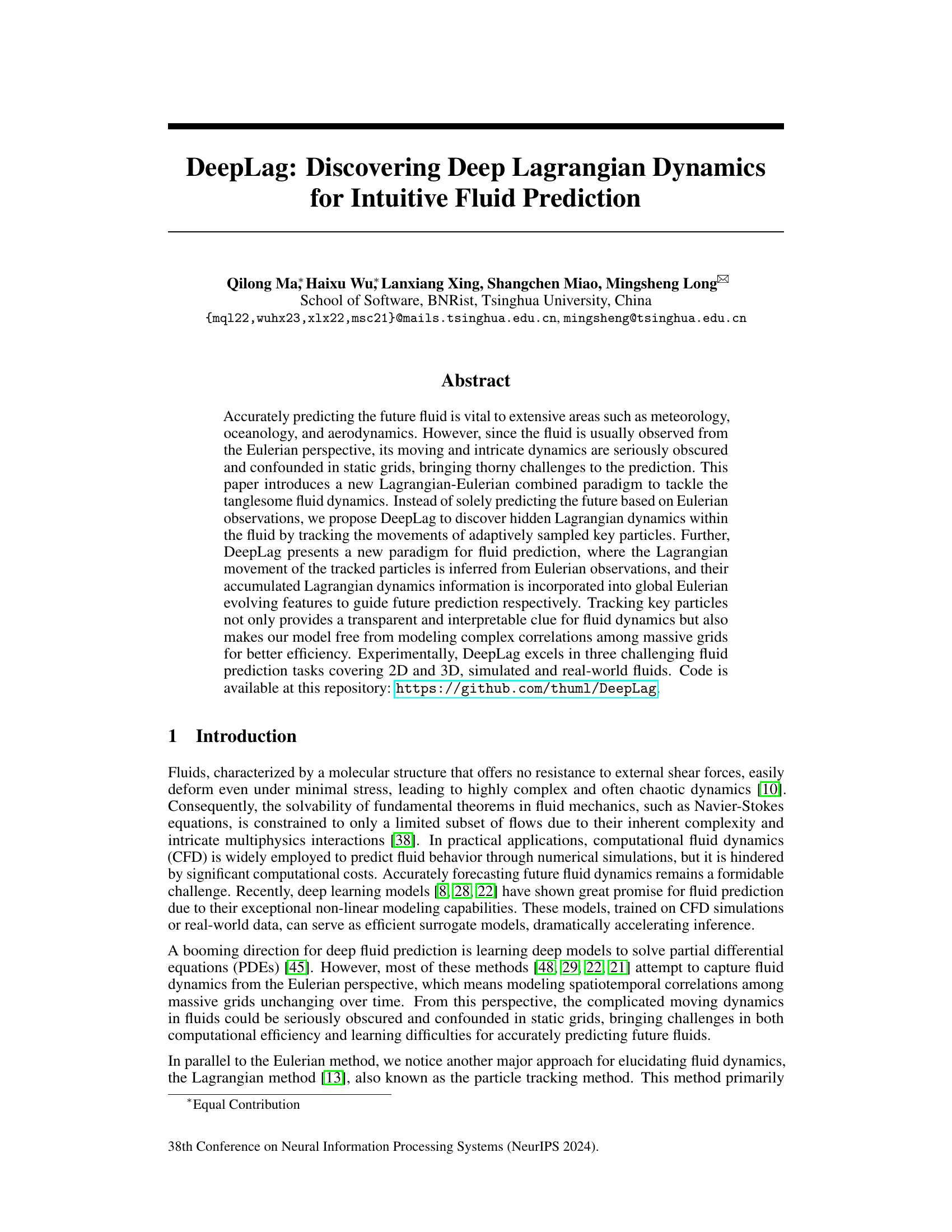
This figure compares Lagrangian and Eulerian perspectives for visualizing fluid motion. The left side shows the learned trajectories of Lagrangian particles overlaid on the average fluid state, highlighting the dynamic nature of the fluid flow. The right side shows the positions of the same particles tracked in successive Eulerian frames (static grids). The contrast demonstrates that the Lagrangian perspective offers a clearer and more intuitive visualization of the fluid’s movement compared to the Eulerian approach which relies on density changes in static grids.

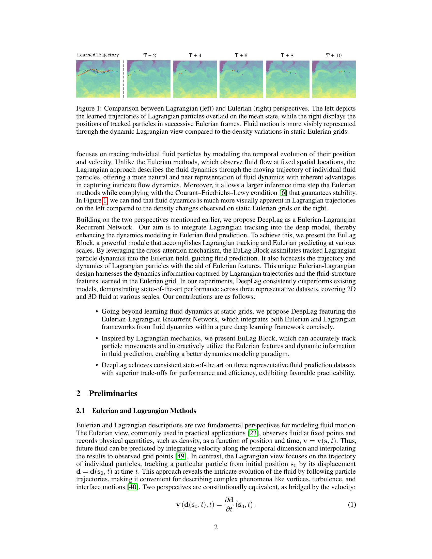
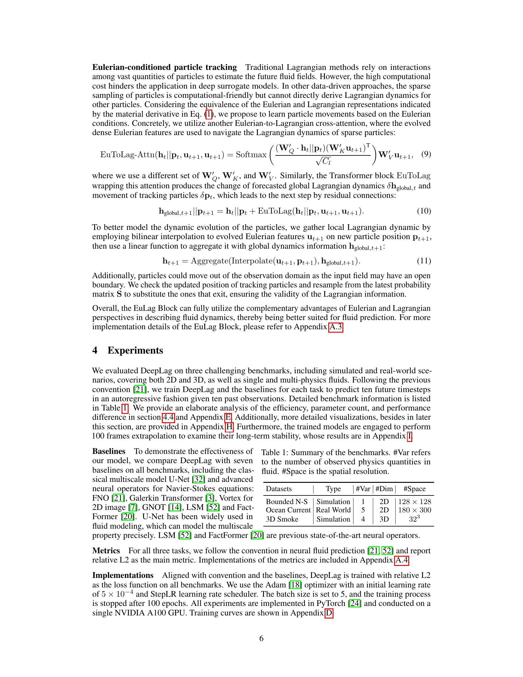
This table summarizes the three benchmark datasets used in the paper to evaluate the DeepLag model and other baselines. It provides key information for each dataset: the type (simulation or real-world), the number of variables (#Var) observed, the dimensionality (#Dim) of the data (2D or 3D), and the spatial resolution (#Space) of the data. This allows readers to understand the nature and scale of the datasets used in the experiments.
In-depth insights#
Lagrangian-Eulerian Fusion#
The concept of ‘Lagrangian-Eulerian Fusion’ in fluid dynamics modeling represents a powerful paradigm shift. Traditional methods heavily rely on either the Eulerian (fixed-grid observation) or Lagrangian (particle tracking) perspective, each with limitations. Eulerian approaches struggle with the inherent complexity of moving fluid dynamics within static grids, often resulting in a loss of crucial information. Conversely, purely Lagrangian methods can be computationally expensive and face challenges in handling large-scale simulations. A fusion approach seeks to synergistically combine the strengths of both. By integrating Lagrangian particle tracking to capture the detailed movement of key fluid elements and subsequently incorporating this dynamic information into a global Eulerian framework, models can achieve significantly improved accuracy and efficiency. The key is the intelligent selection of tracked particles, possibly guided by a learned approach, which enables the capture of essential dynamic information without computational overload. This combined strategy offers a more intuitive and interpretable representation of fluid behaviour, leading to enhanced predictive capabilities, especially in scenarios featuring complex interactions and spatiotemporal correlations, such as turbulent flows and multiphase phenomena.
DeepLag Architecture#
The DeepLag architecture cleverly integrates Eulerian and Lagrangian perspectives for fluid prediction. Eulerian features, extracted from static grid observations, are combined with Lagrangian dynamics learned by tracking key particles. The core innovation is the EuLag Block, which seamlessly fuses these perspectives using cross-attention mechanisms. This allows the model to capture both global spatiotemporal patterns from Eulerian data and detailed local dynamics from Lagrangian particle trajectories. The multiscale design further enhances the model’s ability to represent fluid behavior across different scales. The architecture avoids the computational expense of explicitly modeling complex correlations among massive grids by focusing on key particles. This makes DeepLag more efficient and transparent while maintaining state-of-the-art accuracy, particularly advantageous for long-term predictions.
Multiscale Fluid Dynamics#
Multiscale fluid dynamics is a crucial area of research because fluids exhibit vastly different behaviors across a range of spatial and temporal scales. From the microscopic scale of individual molecules to the macroscopic scale of weather patterns, understanding how these scales interact is essential for accurate modeling and prediction. DeepLag addresses this multiscale nature by employing a novel Eulerian-Lagrangian approach. This integration allows for capturing both global, macroscopic dynamics (Eulerian) and local, microscopic features (Lagrangian) which are essential to represent the complexity of real-world fluid systems. The effectiveness of DeepLag in handling various scales is demonstrated by its ability to excel across diverse datasets, including 2D and 3D simulated and real-world fluid systems. This success speaks to the power of the integrated, multiscale modeling approach and its potential for broader application in areas like weather prediction, climate modeling, and industrial fluid dynamics.
Benchmark Results#
A thorough analysis of benchmark results in a research paper necessitates a multifaceted approach. Firstly, clarity in methodology is paramount; the description of the benchmarks used must be precise, outlining datasets, evaluation metrics, and experimental setup. Secondly, comparing against relevant baselines is crucial; the selected baselines should represent the state-of-the-art or significant alternative approaches, enabling a fair comparison and highlighting the novelty of the proposed method. Next, statistical significance needs careful consideration; error bars or confidence intervals should be presented to demonstrate the reliability of the reported results and avoid overfitting or spurious claims. Finally, interpretability of the results is key; the paper should thoroughly explain any trends or discrepancies observed, relating them back to the methods and underlying principles of the research. A well-written ‘Benchmark Results’ section ultimately offers a robust validation of the proposed work, convincingly showcasing its strengths and limitations within the existing research landscape.
Future Directions#
Future research could explore more sophisticated particle tracking methods to better capture complex fluid dynamics, potentially incorporating machine learning techniques to adaptively sample key particles. Improving the model’s ability to handle high-dimensional data and different fluid types would be valuable, along with investigating the model’s robustness under diverse boundary conditions. A promising area involves investigating the incorporation of additional physical constraints and incorporating multi-physics interactions to enhance prediction accuracy. Finally, exploring the model’s interpretability through techniques like attention visualization can lead to a better understanding of how it extracts and combines information from Lagrangian and Eulerian representations. This could lead to more efficient and reliable predictions.
More visual insights#
More on figures
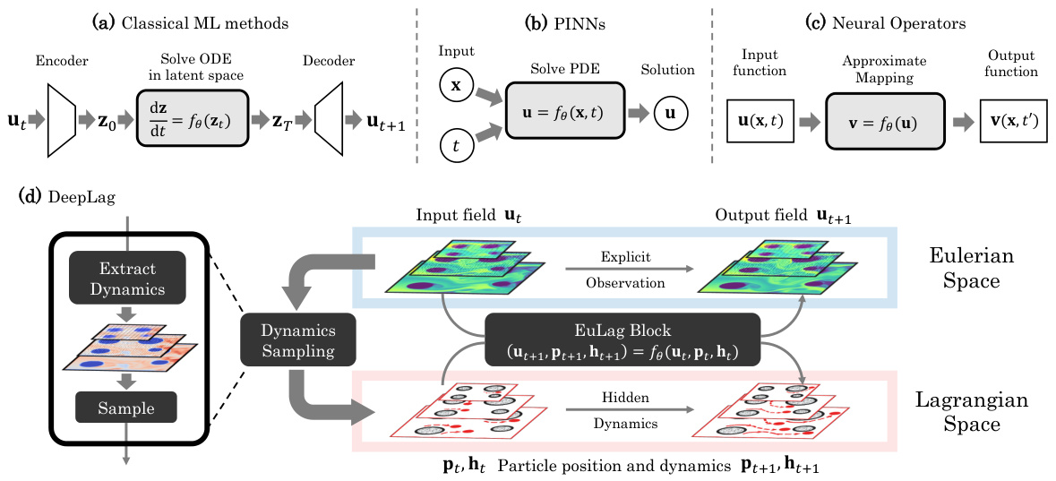
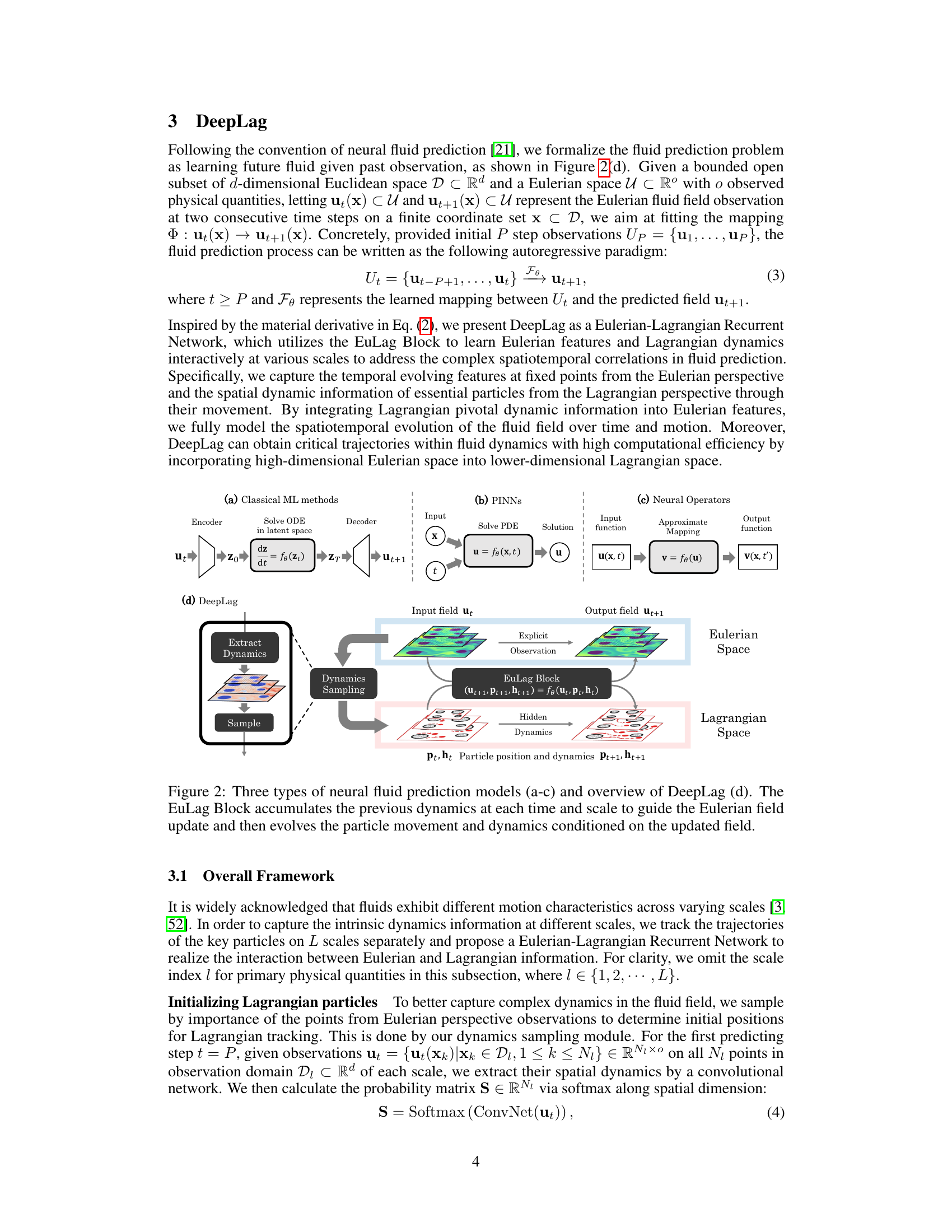
This figure provides a visual comparison of three main neural fluid prediction methods: Classical ML methods, Physics-Informed Neural Networks (PINNs), and Neural Operators. Each method is depicted with a diagram showing its input, process, and output. Additionally, it shows an overview of the proposed DeepLag method, highlighting its unique Eulerian-Lagrangian Recurrent Network and EuLag Block. The EuLag Block is shown to integrate Lagrangian particle tracking with Eulerian field prediction for more accurate and efficient fluid dynamics modeling.

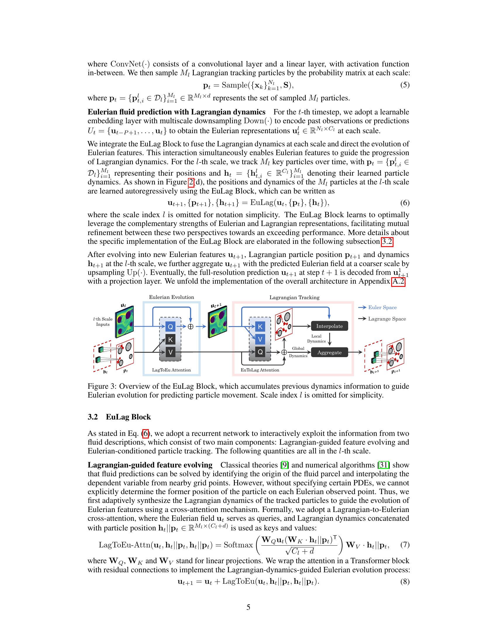
This figure illustrates the EuLag Block, a core component of the DeepLag model. It shows how the model integrates Eulerian (grid-based) and Lagrangian (particle-based) perspectives to predict fluid motion. The EuLag block consists of two main processes: 1. Lagrangian-guided feature evolving: Using cross-attention, Lagrangian particle dynamics (position and learned dynamics) are integrated with Eulerian features to guide the prediction of the next Eulerian field. 2. Eulerian-conditioned particle tracking: Again, using cross-attention, the updated Eulerian field is used to predict the next position and dynamics of the Lagrangian particles. The updated Eulerian field and particle information are then fed back into the recurrent network for the next time step. The process occurs across multiple scales, with information from coarser scales being aggregated into finer scales. The simplified notation omits the scale index ’l’ for clarity.

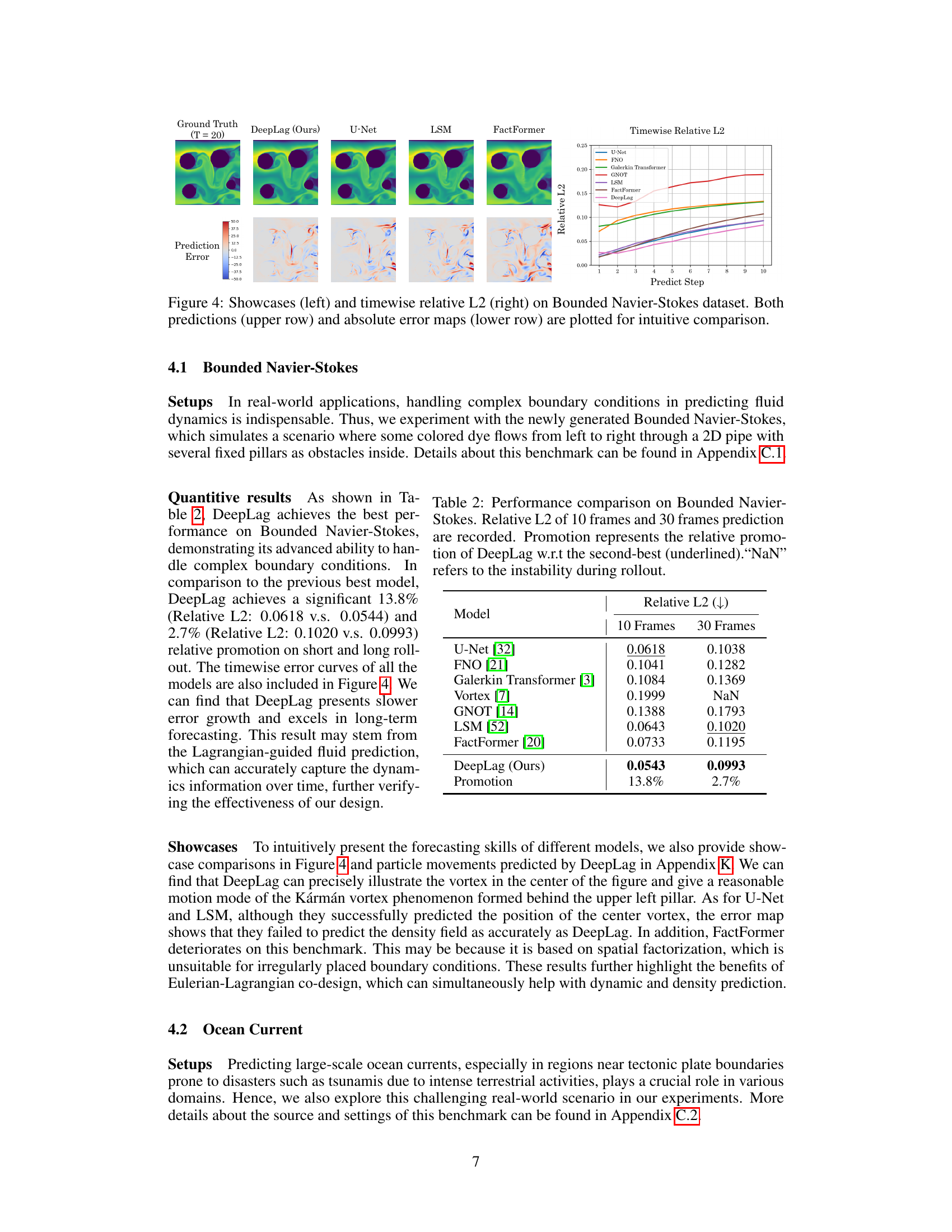
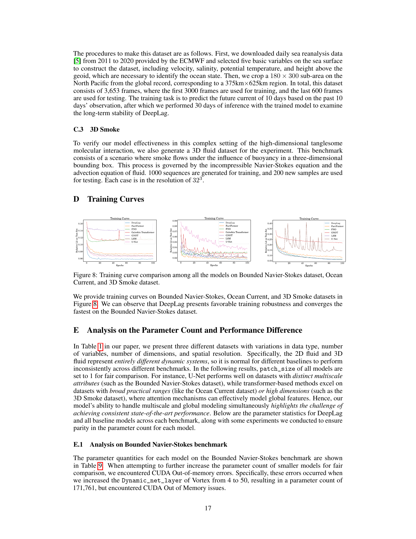
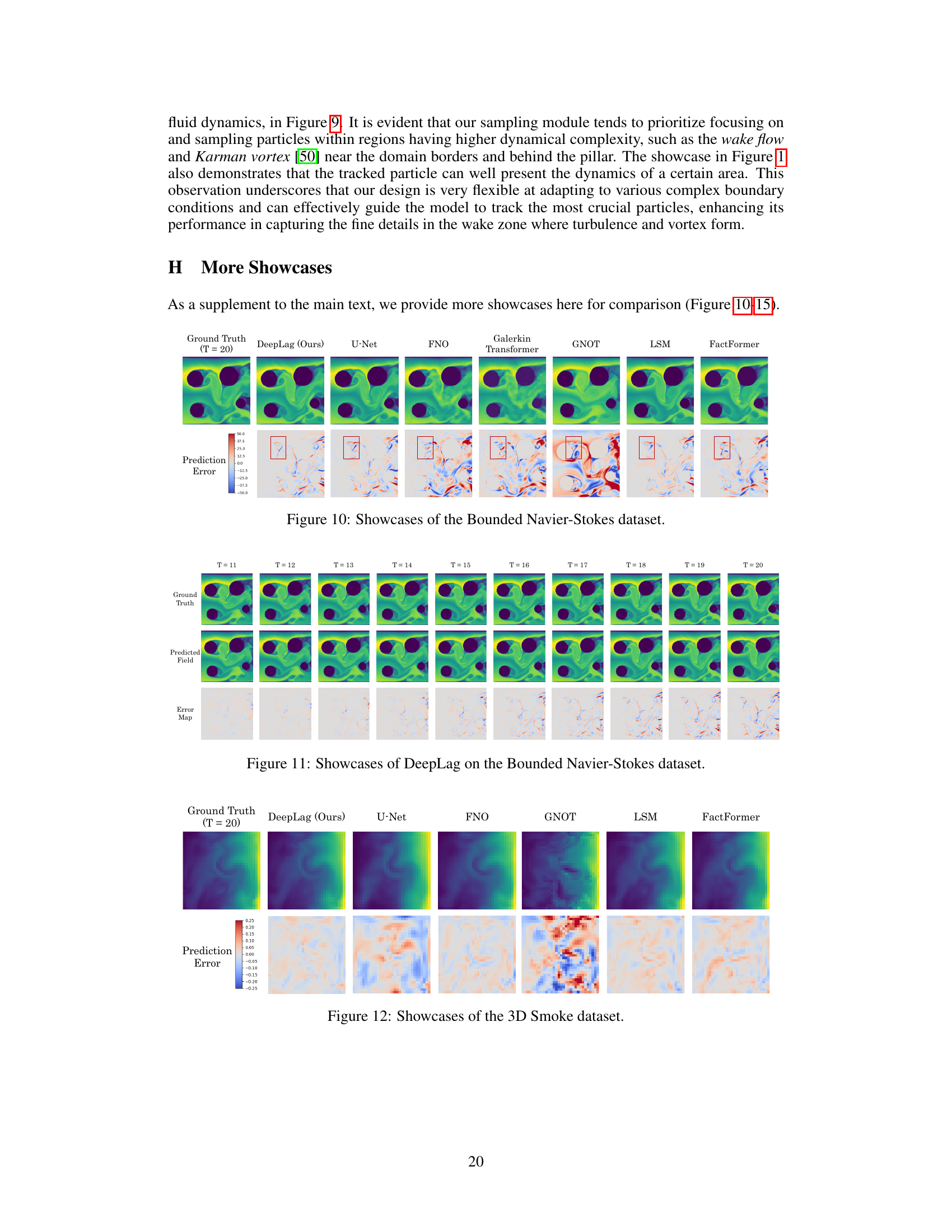
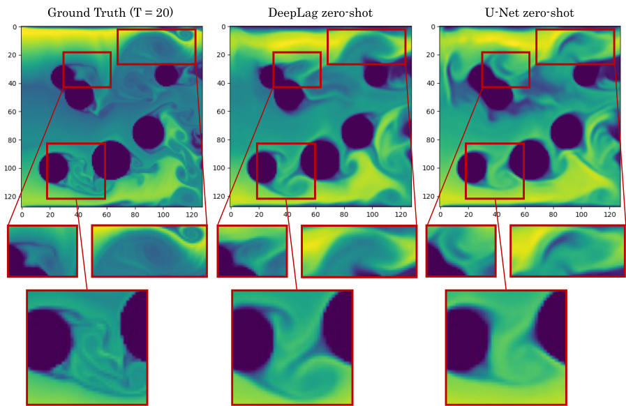
This figure shows a comparison of the DeepLag model’s performance against other baseline models on the Bounded Navier-Stokes dataset. The left side showcases the ground truth, DeepLag prediction, and predictions from other models at a specific time step (T=20). The right side shows the timewise relative L2 error, illustrating the model’s performance over time for predicting the fluid’s evolution. The visualization helps assess each model’s ability to accurately capture the complex fluid dynamics and boundary conditions of this challenging dataset.

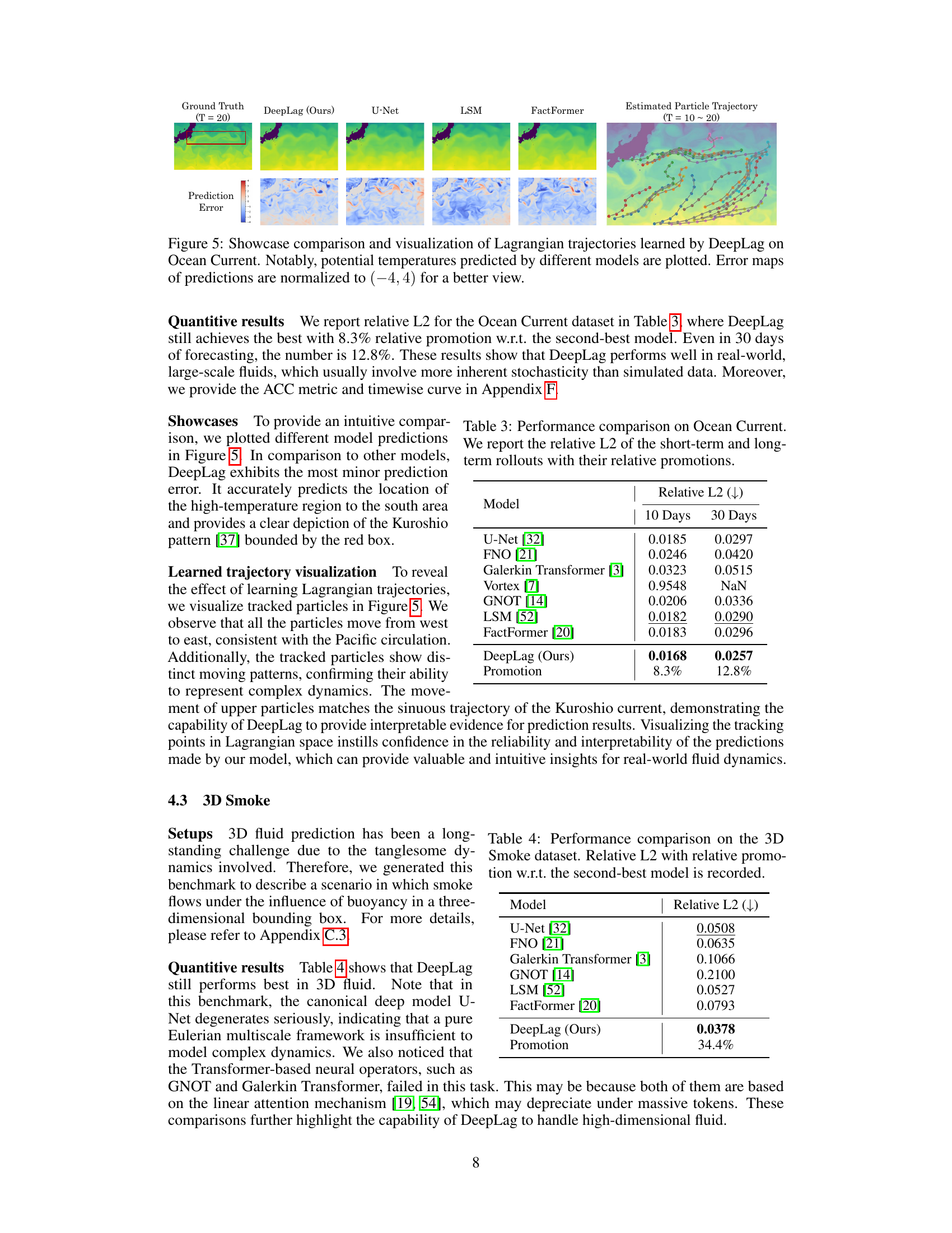
This figure compares the prediction results of DeepLag and other models on the Ocean Current dataset. The left side shows the ground truth, DeepLag’s prediction, and the predictions of three other models (U-Net, LSM, and FactFormer). The right side visualizes the trajectories of particles learned by DeepLag, overlaid on the potential temperature field. Error maps are provided for a visual comparison of the predictions.

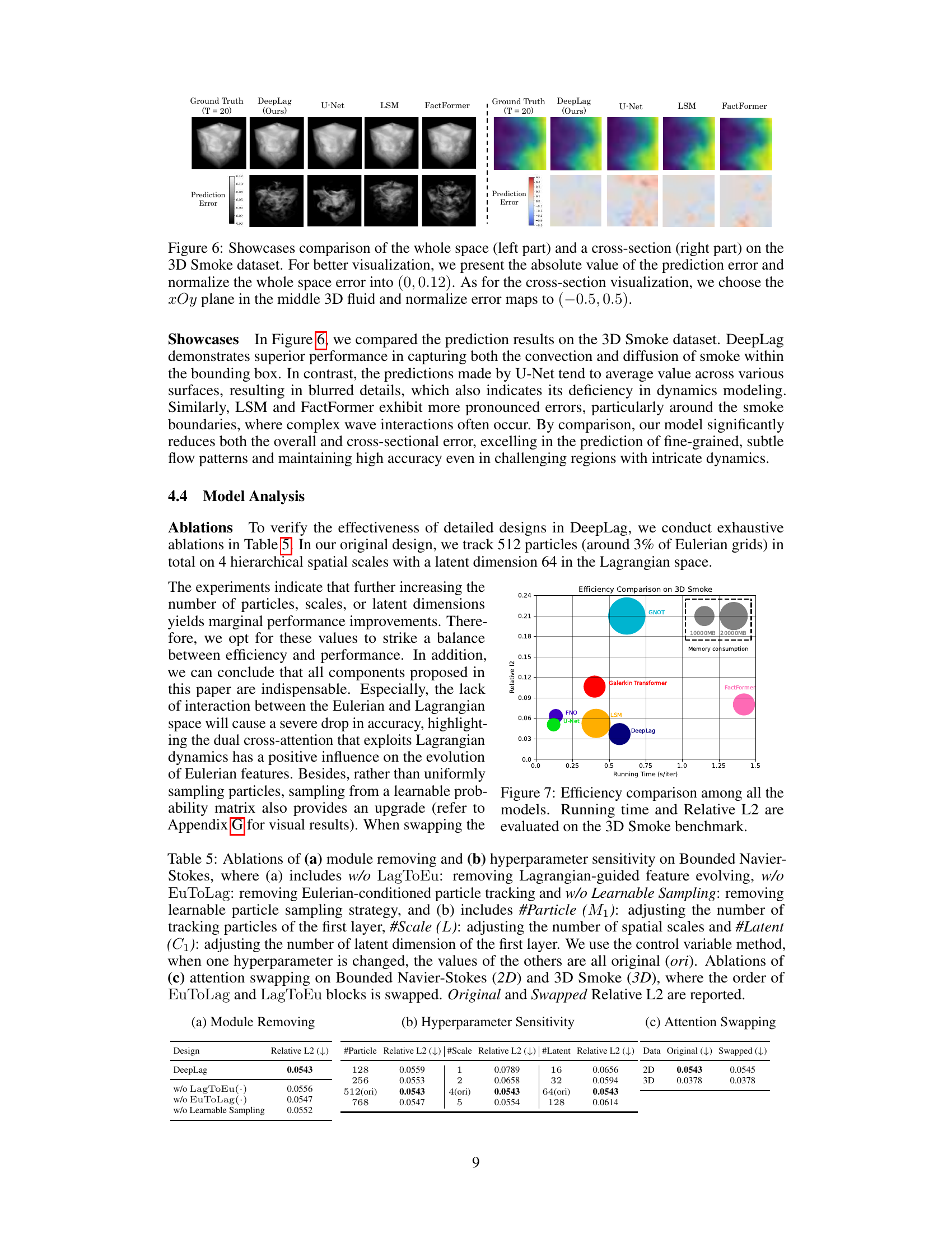
This figure compares the prediction results of different models on the 3D Smoke dataset. It shows the whole space prediction and a cross-section (xOy plane) for better visualization. The absolute prediction error is normalized for better comparison.
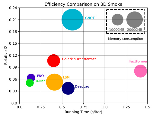
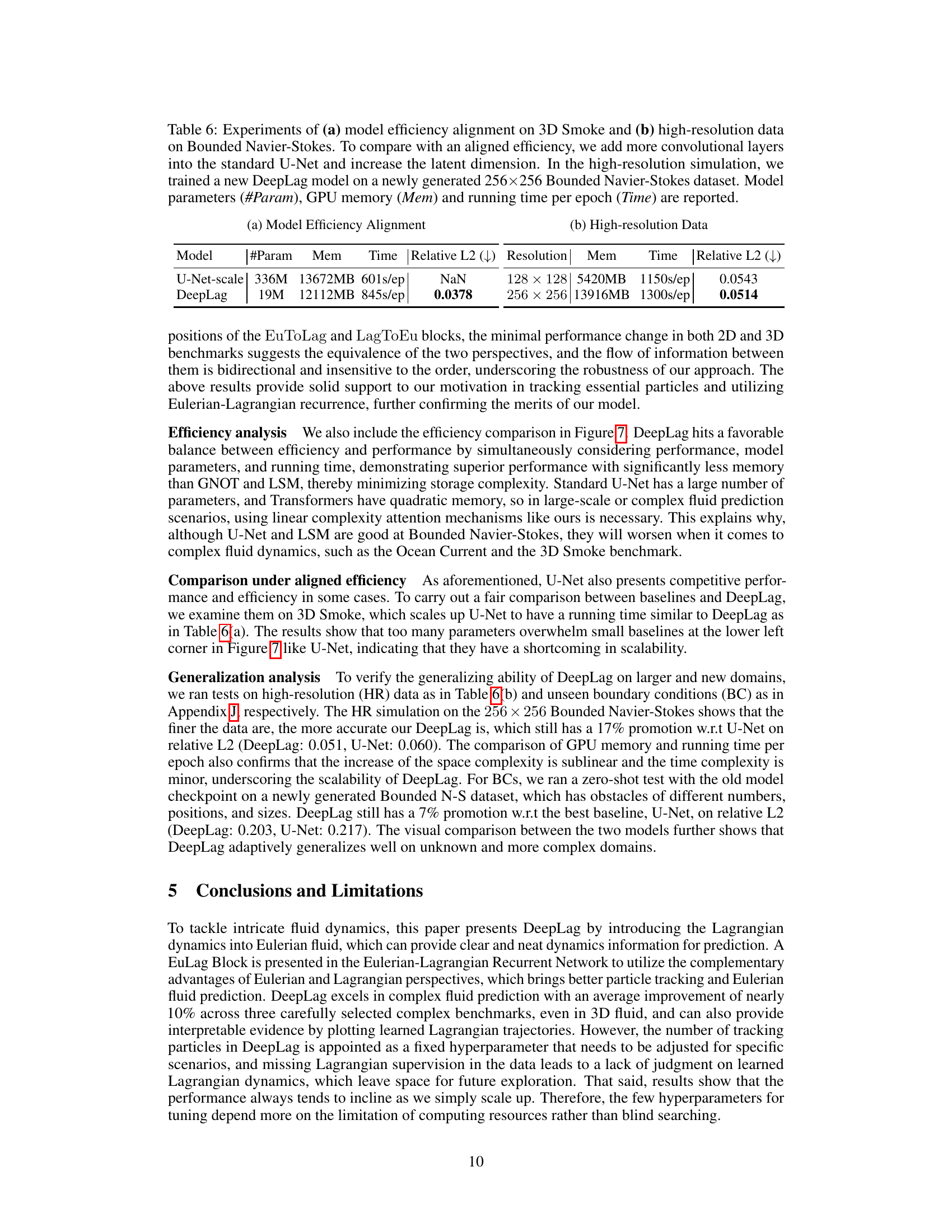
This figure compares seven different neural network models for fluid prediction on the 3D Smoke dataset. The comparison is made based on two metrics: running time per iteration and relative L2 error. The size of each circle represents the memory consumption of the model. DeepLag shows a favorable balance between efficiency and accuracy.

This figure compares three main types of neural fluid prediction models and introduces the proposed DeepLag model. (a-c) show classical machine learning methods, physics-informed neural networks, and neural operators respectively. These approaches are compared to (d) the DeepLag architecture which uses an EuLag block to integrate Eulerian and Lagrangian information for fluid prediction. The EuLag block combines the temporal evolution of Eulerian features at fixed points with the spatial dynamics of adaptively sampled key particles through their movements to guide the Eulerian and Lagrangian updates iteratively.

This figure presents a comparison of the model’s performance on the Bounded Navier-Stokes dataset. The left panel showcases the ground truth, DeepLag predictions, and predictions from several other models, allowing for a visual comparison of the results. The right panel shows the relative L2 error over time for each model, which quantifies the prediction accuracy. Both predictions and absolute error maps are displayed for a more comprehensive understanding of the model’s performance.

This figure shows a comparison of the predictions of different models on the Bounded Navier-Stokes dataset. The left part shows the prediction results of different models, including DeepLag, U-Net, FNO, Galerkin Transformer, GNOT, LSM, and FactFormer, and the corresponding ground truth. The right part shows the timewise relative L2 error for these models. The error maps are also shown to provide a visual comparison of the prediction errors. DeepLag is shown to have superior performance compared to the other models.

This figure compares Lagrangian and Eulerian perspectives on fluid prediction. The left side shows the learned trajectories of Lagrangian particles, highlighting their movement and dynamic nature. In contrast, the right side uses static Eulerian grids to display tracked particle positions in successive frames, showcasing the limitations of Eulerian perspectives. The comparison visually demonstrates that the Lagrangian view provides a clearer and more informative representation of fluid motion compared to Eulerian grids.

This figure presents a qualitative and quantitative comparison of different fluid prediction models on the Bounded Navier-Stokes dataset. The left side shows visual showcases of the ground truth, DeepLag’s prediction, and predictions from other models (U-Net, FNO, Galerkin Transformer, GNOT, LSM, FactFormer). The right side displays a graph showing the timewise relative L2 error across different prediction steps for each model. This allows for a visual and numerical assessment of the models’ performance.

This figure showcases a comparison of the potential temperature predictions of different models on the Ocean Current dataset. DeepLag’s prediction is visually compared to the ground truth and other models (U-Net, LSM, FactFormer). The figure also includes a visualization of the Lagrangian trajectories learned by DeepLag, highlighting the movement of particles in the dataset. Error maps are displayed to provide a quantitative comparison. The normalization to (-4, 4) enhances the clarity of the error maps.
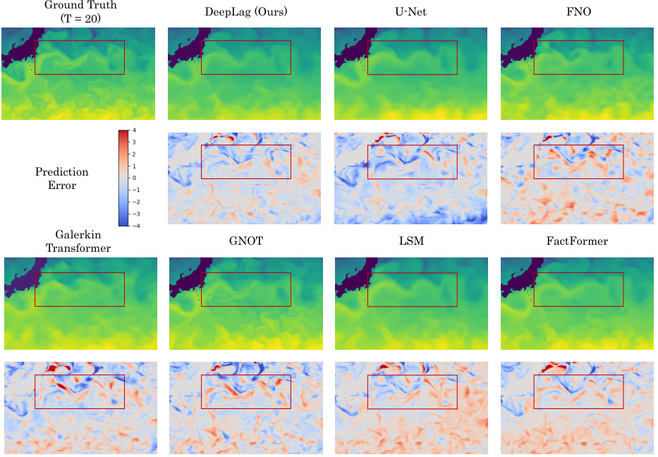
This figure showcases a comparison of different models’ predictions for ocean currents, including DeepLag. It visually demonstrates the accuracy of each model’s predictions by comparing them to the ground truth. In addition to the predictions themselves, Lagrangian particle trajectories (learned by DeepLag) and potential temperature predictions are also shown for a more intuitive understanding of fluid dynamics. The error maps provide a quantitative assessment of the prediction accuracy.
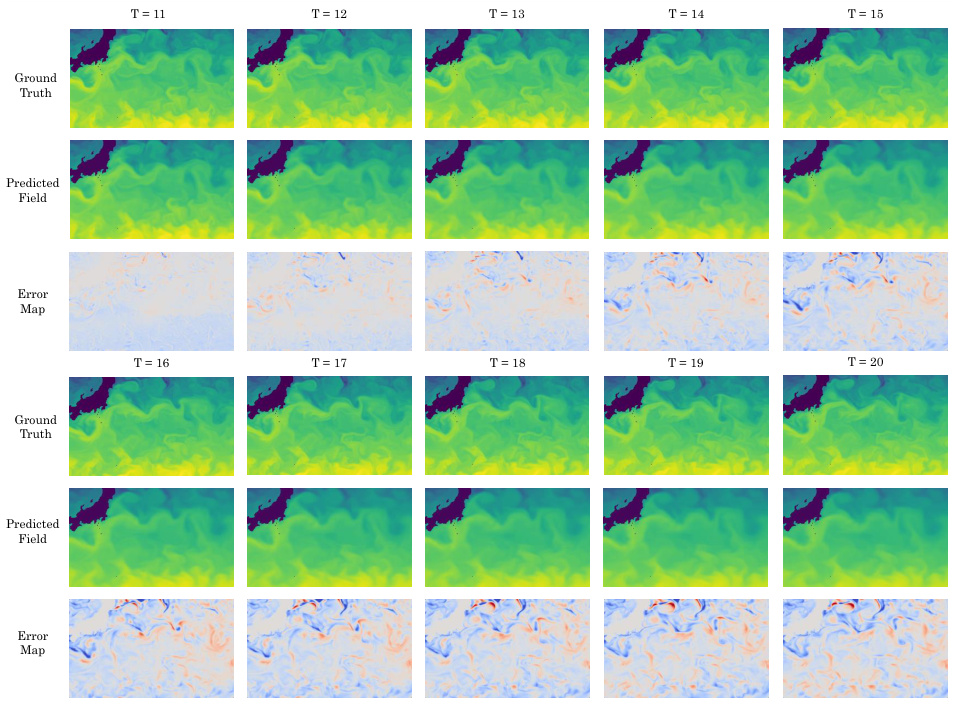
This figure showcases a comparison of the potential temperature predictions from different models on the Ocean Current dataset. It highlights DeepLag’s superior accuracy by comparing its predictions to those of other models. The visualization includes the ground truth, DeepLag’s prediction, and the predictions from several other models. Lagrangian trajectories, learned by DeepLag, are also visualized, providing further insight into the model’s approach.
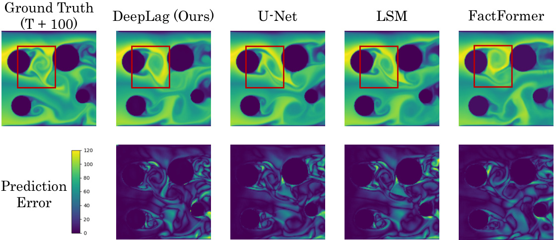
This figure compares the long-term prediction results (T=100) of DeepLag, U-Net, LSM, and FactFormer on the Bounded Navier-Stokes dataset. The top row shows the ground truth and the predictions of each model, while the bottom row displays the absolute error maps for each prediction. The red boxes highlight areas of interest for visual comparison. The results demonstrate DeepLag’s superior performance in predicting the complex flow patterns and vortex structures compared to other models.

This figure compares Lagrangian and Eulerian perspectives on fluid prediction. The left side shows the trajectory of Lagrangian particles, highlighting the fluid motion more clearly than the right side which shows the particles in successive Eulerian frames, where fluid motion is less apparent.

This figure compares Lagrangian and Eulerian perspectives for visualizing fluid motion. The left side shows the learned trajectories of Lagrangian particles, providing a dynamic view of their movement through the fluid. In contrast, the right side shows the particle positions in successive Eulerian frames (static grids), revealing a less clear picture of the fluid motion. The comparison demonstrates that the Lagrangian perspective offers a more intuitive representation of fluid dynamics.

This figure shows the timewise results of DeepLag’s long-term prediction on the Bounded Navier-Stokes dataset. It displays the ground truth, the model’s prediction, and the error map for each time step (T+0 to T+100). This visualization allows for a clear comparison of the model’s performance over an extended period and highlights its ability to capture complex fluid dynamics.

This figure displays a time series of predictions from DeepLag on the Bounded Navier-Stokes dataset. Each column represents a specific time step, ranging from T+0 to T+100. The top row presents the ground truth, the middle row shows DeepLag’s prediction, and the bottom row shows the error map comparing the prediction to the ground truth. The figure highlights DeepLag’s ability to maintain accuracy over a long time frame (100 time steps) in this challenging scenario.

This figure showcases a comparison of long-term prediction results (at T=100) on the Ocean Current dataset, comparing DeepLag against U-Net, LSM, and FactFormer. The top row shows the ground truth at T=100, and the bottom row shows the prediction error. Each column represents a different model’s prediction, allowing for a visual comparison of accuracy and error patterns.

This figure compares Lagrangian and Eulerian perspectives on fluid motion prediction. The left side shows the trajectories of tracked particles (Lagrangian), highlighting the dynamic nature of the fluid flow. The right side shows the particles’ positions at successive time steps in a static grid (Eulerian), making the fluid motion less obvious. This illustrates the advantage of the Lagrangian approach in visualizing fluid dynamics.

This figure compares Lagrangian and Eulerian perspectives on fluid motion prediction. The left side shows the learned trajectories of Lagrangian particles, highlighting how their movement represents fluid dynamics more clearly than the density variations in static Eulerian grids shown on the right side.

This figure shows a time series of predictions from the LSM model on the Ocean Current dataset, which includes ground truth, prediction, and error map. Each column represents the prediction for a given time step (T+0 to T+100), showcasing the model’s ability to predict ocean current patterns over a longer time horizon.

This figure compares the long-term prediction results (100 time steps) of DeepLag, U-Net, LSM, and FactFormer on the Bounded Navier-Stokes dataset. It shows the ground truth at T+100, the predictions of each model, and the corresponding error maps. The purpose is to visually demonstrate the long-term prediction capabilities of each model and compare DeepLag’s performance against other leading methods, particularly regarding its ability to maintain accuracy over an extended prediction horizon.

This figure presents a qualitative and quantitative comparison of different models’ performance on the Bounded Navier-Stokes dataset. The left part showcases the ground truth, predictions by DeepLag and other models, and their corresponding error maps for a visual comparison of the flow patterns. The right part displays the timewise relative L2 error curves for each model, providing a quantitative assessment of their prediction accuracy over time.
This figure showcases a comparison between the ground truth and predictions made by DeepLag, U-Net, LSM, and FactFormer on the 3D Smoke dataset. The left side shows the whole space, visualizing the absolute prediction errors normalized to a range of (0, 0.12). The right side shows a cross-section (xOy plane in the middle of the 3D space), with prediction errors normalized to (-0.5, 0.5). The visualization highlights DeepLag’s superior performance in capturing fine-grained details and accurately predicting the smoke’s flow compared to the other models.
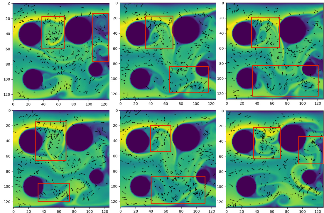
This figure compares the Lagrangian and Eulerian perspectives for visualizing fluid motion. The left panel shows the learned trajectories of Lagrangian particles overlaid on the mean fluid state, highlighting the dynamic nature of the fluid. The right panel shows the positions of the same particles in a series of static Eulerian grids, demonstrating how the intricate fluid dynamics is obscured in this static representation. The comparison emphasizes the advantages of the Lagrangian perspective in clearly visualizing fluid movement.
More on tables
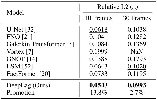
This table presents a comparison of the performance of DeepLag against several baseline models on the Bounded Navier-Stokes dataset. The metrics used are Relative L2 error for both 10-frame and 30-frame predictions. The ‘Promotion’ column indicates the percentage improvement of DeepLag’s performance compared to the second-best performing model. ‘NaN’ signifies that a model was unstable and could not complete the 30-frame prediction.
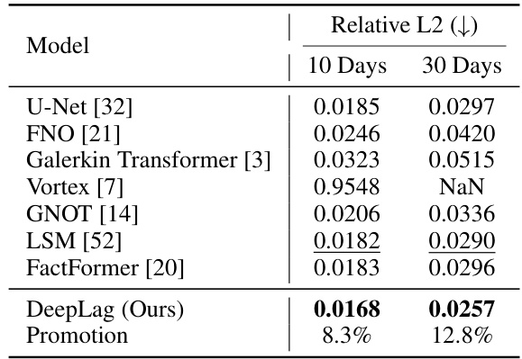
This table presents a comparison of the performance of different models on the Ocean Current dataset in terms of Relative L2 error for both short-term (10 days) and long-term (30 days) predictions. The ‘Promotion’ row indicates the percentage improvement of DeepLag over the second-best performing model for each prediction horizon. Lower Relative L2 values indicate better predictive accuracy.
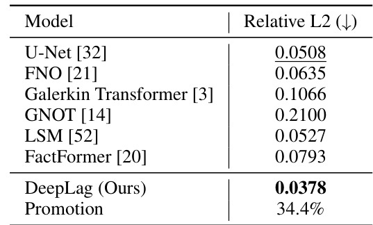
This table presents a comparison of the performance of DeepLag and several baseline models on the 3D Smoke dataset. The key metric is Relative L2, showing how much better DeepLag performs compared to other models. The ‘Promotion’ column indicates the percentage improvement of DeepLag relative to the second-best performing model.

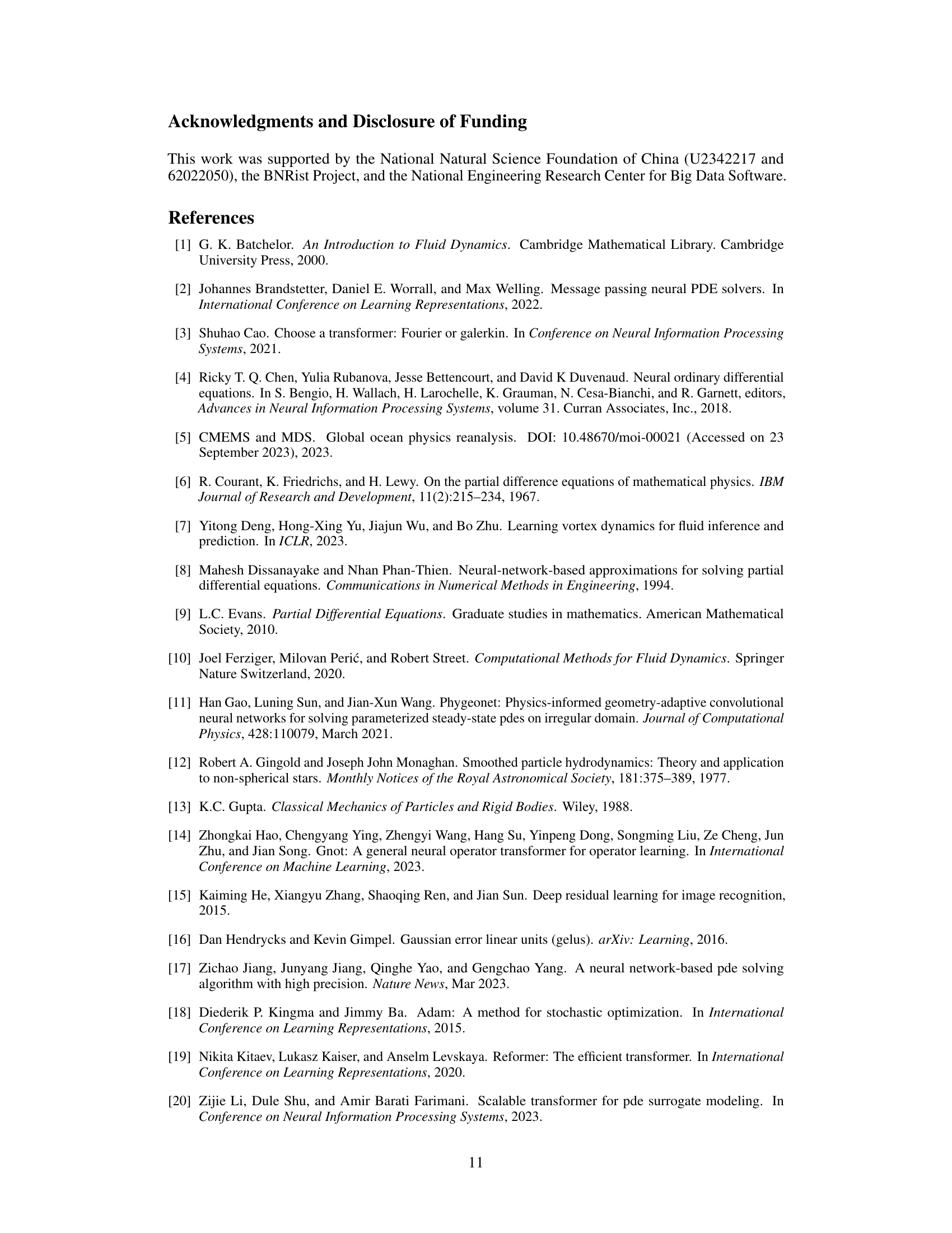
This table presents ablation studies on the DeepLag model. It shows the impact of removing different components of the model (LagToEu, EuToLag, and Learnable Sampling) and varying hyperparameters (#Particle, #Scale, #Latent) on the model’s performance (Relative L2). It also tests swapping the order of the attention mechanisms (LagToEu and EuToLag). The results highlight the importance of each component for the model’s effectiveness and the robustness of the attention mechanism order.

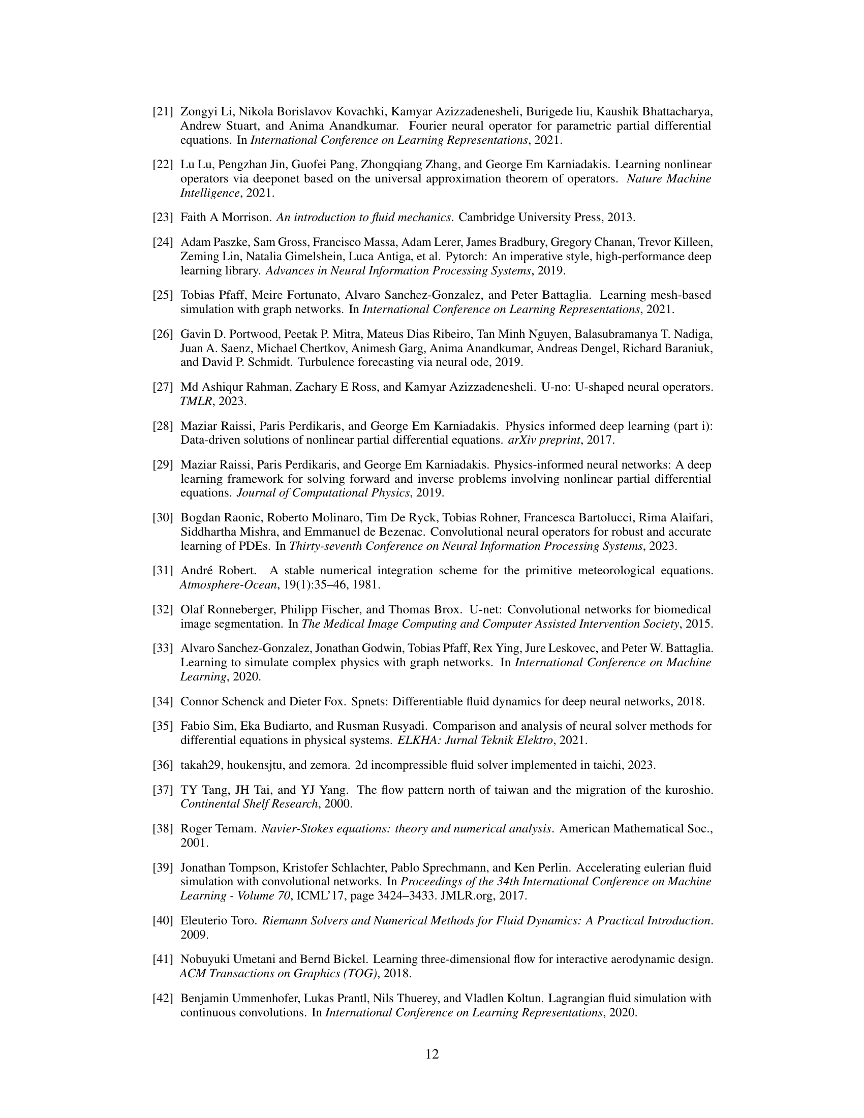
This table compares the efficiency and performance of DeepLag and a modified U-Net model on two different scenarios: efficiency alignment (3D Smoke dataset) and high-resolution data (Bounded Navier-Stokes dataset). The modified U-Net model has increased parameters and latent dimension to match DeepLag’s running time. The table shows the number of parameters, GPU memory usage, running time per epoch, and relative L2 error for both models in each scenario. It highlights DeepLag’s computational efficiency and performance, even on high-resolution data.
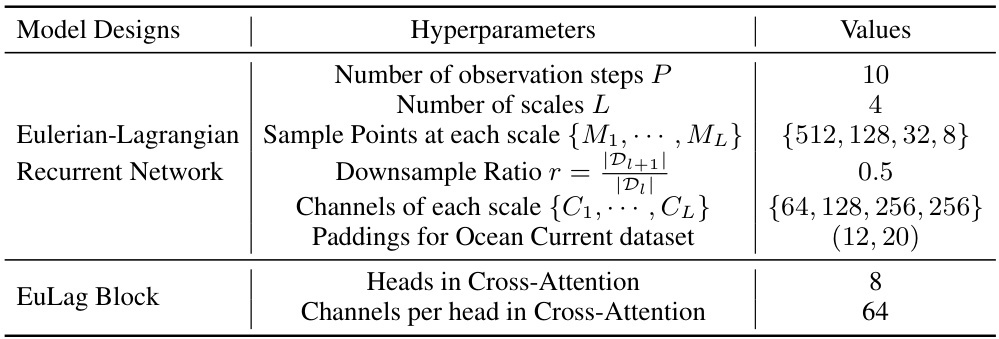
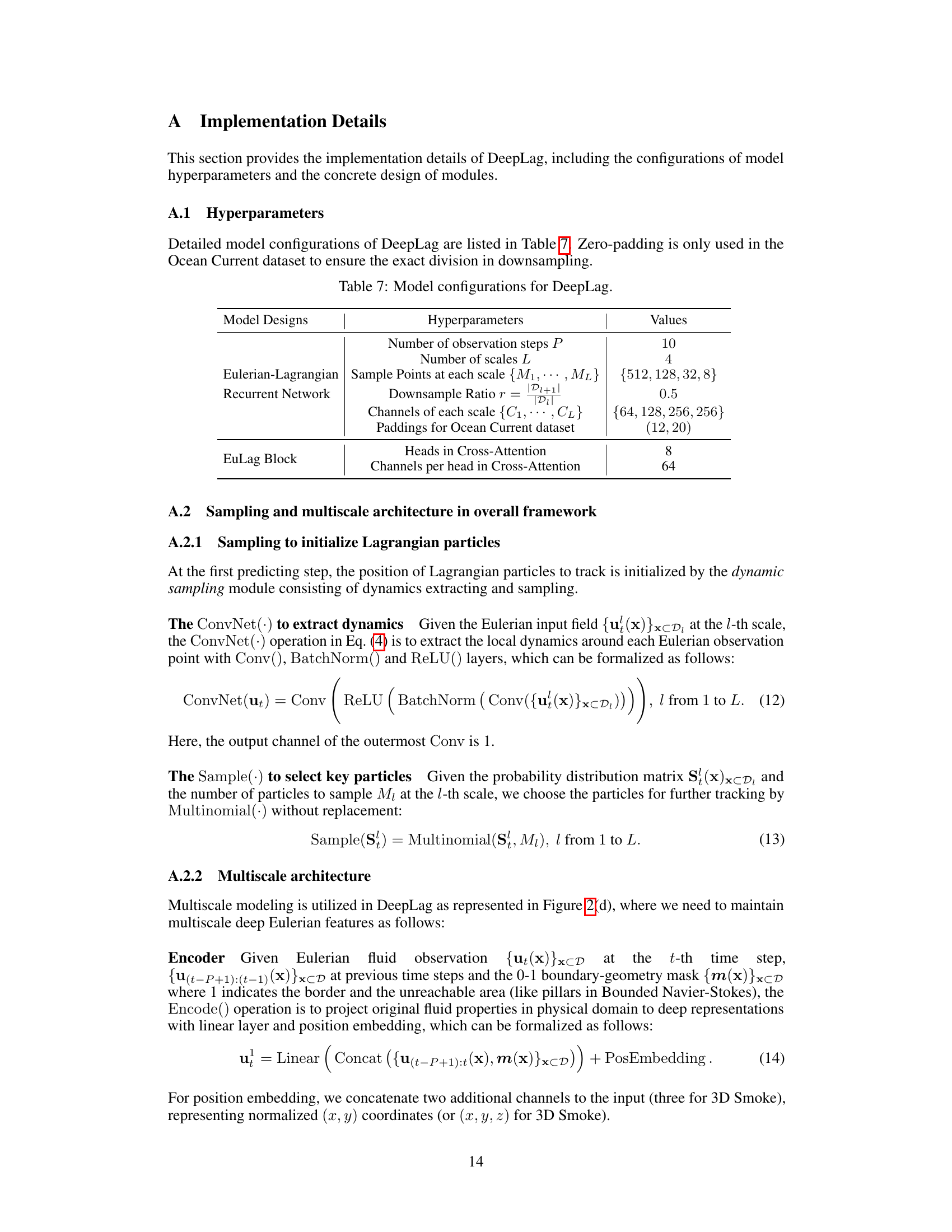
This table lists the hyperparameters used in the DeepLag model. It specifies the number of observation steps, number of scales used in the multiscale architecture, the number of sample points at each scale for Lagrangian tracking, the downsample ratio between scales, the number of channels in each scale for Eulerian features, and padding used for the Ocean Current dataset. It also provides details of hyperparameters related to the EuLag Block, including the number of heads and channels per head in the cross-attention mechanism.

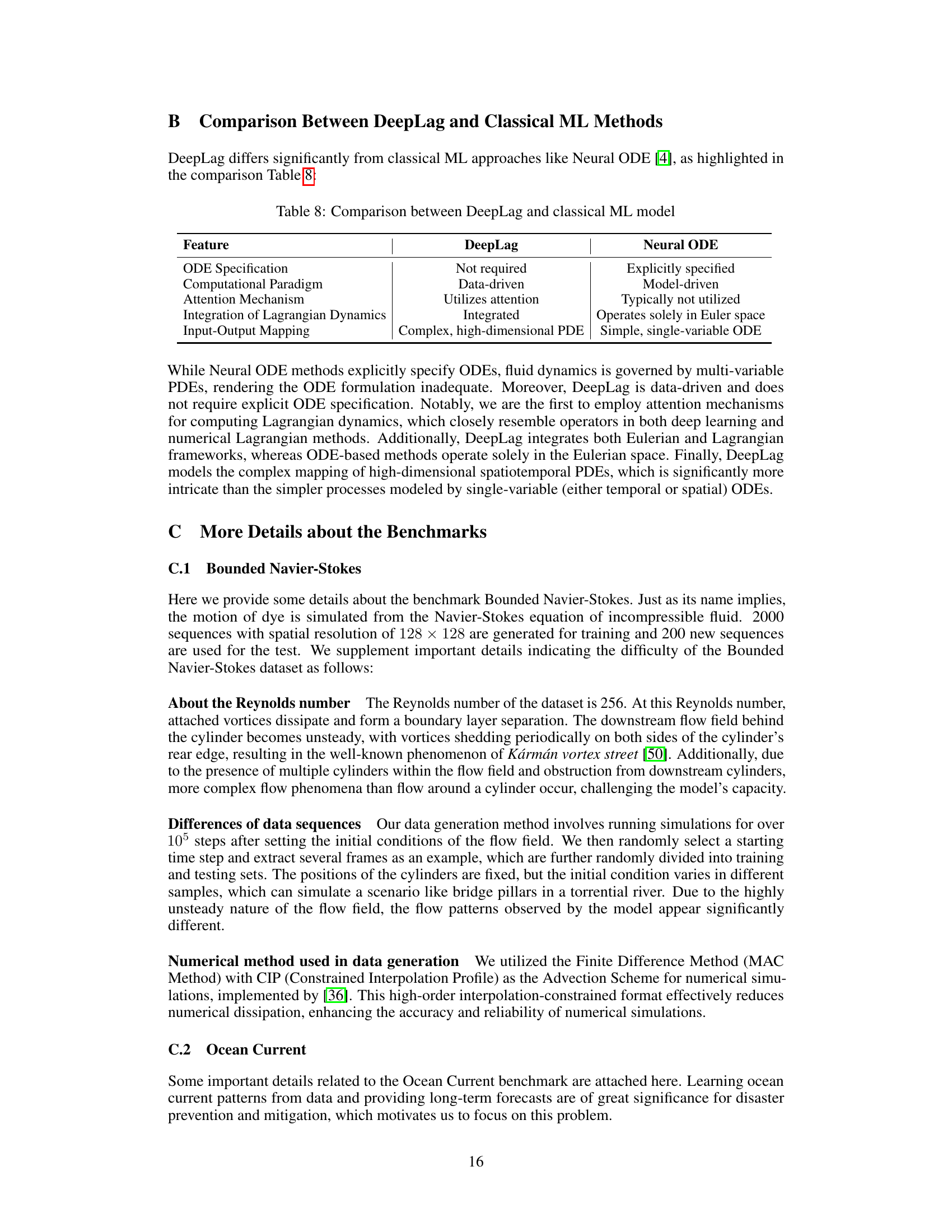
This table compares DeepLag with Neural ODE methods. It highlights key differences in ODE specification (whether an ODE is explicitly required or not), the computational paradigm (data-driven vs. model-driven), the use of attention mechanisms, the integration of Lagrangian dynamics, and the input-output mapping complexity. The table shows that DeepLag is data-driven, uses attention, integrates Lagrangian dynamics, and handles complex, high-dimensional PDEs, unlike Neural ODE which is model-driven, typically doesn’t use attention, operates solely in Eulerian space, and handles simpler, single-variable ODEs.
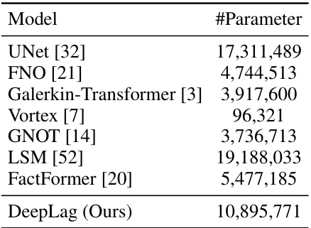
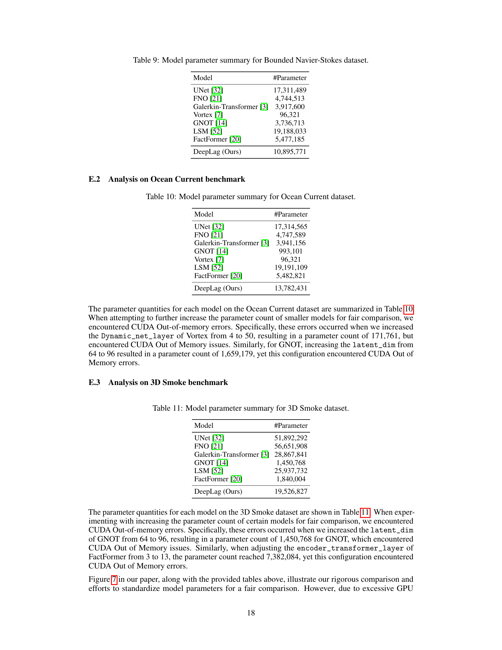
This table presents the number of parameters for each model used in the Bounded Navier-Stokes experiment. The models are compared for performance, and this data helps understand the model complexity. The table shows a wide range of parameter counts, highlighting differences in model architecture and capacity.
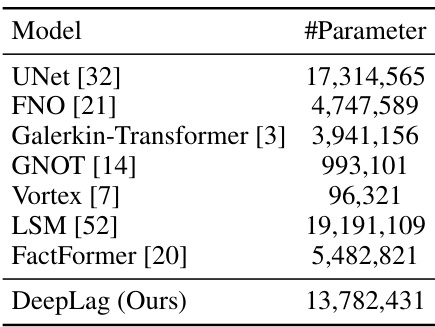
This table presents a comparison of the number of parameters for different models used in the Ocean Current benchmark. It helps illustrate the relative model complexity and potential computational resource requirements.
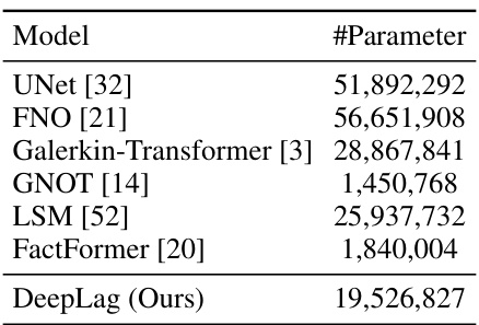
This table presents the number of parameters for each model on the 3D Smoke dataset. It compares DeepLag’s parameter count with seven other baseline models (UNet, FNO, Galerkin-Transformer, GNOT, LSM, FactFormer). The table highlights the relative efficiency of DeepLag compared to more parameter-heavy models.

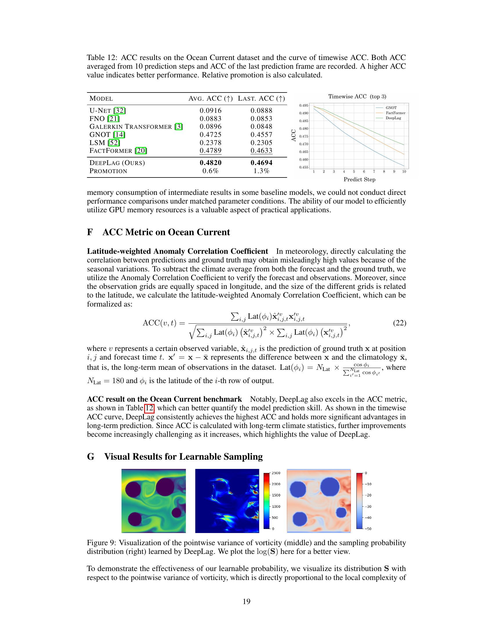
This table presents the results of the Anomaly Correlation Coefficient (ACC) metric on the Ocean Current dataset. It compares the performance of DeepLag against several baseline models, reporting both the average ACC over 10 prediction steps and the ACC of the final prediction step. A line graph visualizing the timewise ACC is also included. Higher ACC values indicate better performance; relative improvements are calculated comparing DeepLag against the best performing baseline model.
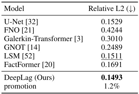
This table shows a performance comparison of DeepLag and seven baseline models on the task of predicting 100 frames into the future for the Bounded Navier-Stokes dataset. The metric used is Relative L2 error. DeepLag achieves the best performance with a 1.2% improvement over the second-best model. The table highlights DeepLag’s superior performance in long-term prediction.
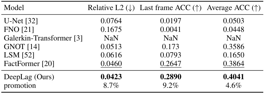
This table presents a comparison of results for the Ocean Current dataset. It shows the Relative L2 error (lower is better) for predicting 100 frames into the future, along with the Last frame ACC (higher is better) and the Average ACC (higher is better) across all 10 prediction steps. The ‘promotion’ row indicates the percentage improvement of DeepLag’s performance compared to the second-best performing model.
Full paper#
