↗ OpenReview ↗ NeurIPS Homepage ↗ Chat
TL;DR#
Diffusion models have achieved state-of-the-art results in image generation, but their strong generalization ability remains poorly understood. Existing theoretical analyses rely on simplified assumptions about data distribution and model architecture, failing to capture the complexities of real-world scenarios where models are trained on finite datasets. This paper investigates the hidden properties of the learned score functions in diffusion models to gain insights into their generalizability.
The researchers employed a linear distillation approach to approximate the nonlinear diffusion denoisers with linear models. They found that in the generalization regime, diffusion models exhibit an inductive bias towards learning Gaussian structures (characterized by empirical mean and covariance of training data). This bias is more pronounced when model capacity is relatively small compared to the dataset size and emerges in early training even in overparameterized models. The study connects this Gaussian bias to the phenomenon of “strong generalization”, where models trained on distinct datasets generate similar outputs. The findings challenge existing theoretical understandings and offer crucial insights for designing more efficient and generalizable diffusion models.
Key Takeaways#
Why does it matter?#
This paper is crucial for researchers in generative modeling as it reveals the hidden inductive bias of diffusion models towards Gaussian structures, particularly impacting understanding generalization and improving model training. It challenges existing assumptions, prompting new research avenues on architectural design and training strategies to leverage this bias.
Visual Insights#
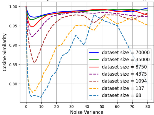
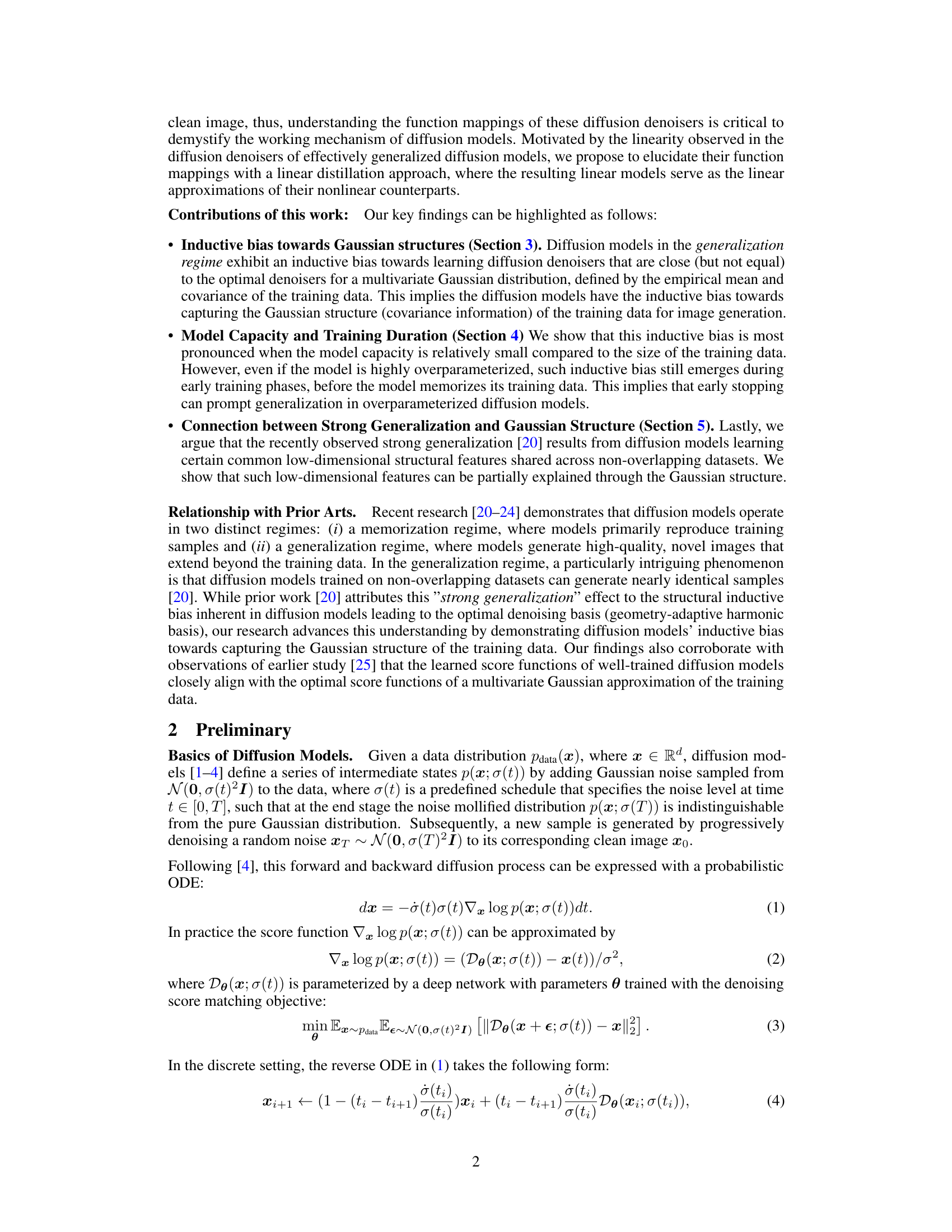
This figure shows how the linearity of diffusion denoisers changes with different training dataset sizes. The linearity score is calculated using cosine similarity, measuring how close the denoiser’s output is to a linear combination of its inputs. The solid lines represent models that have generalized well to unseen data, showing increased linearity as the dataset size increases. The dashed lines show models in the memorization phase where they primarily replicate the training data, exhibiting lower linearity. The x-axis represents the noise variance and the y-axis represents the linearity score. The plot demonstrates a clear trend: models trained on larger datasets exhibit greater linearity and hence better generalization capabilities.
In-depth insights#
Diffusion’s Linearity#
The concept of “Diffusion’s Linearity” unveils a surprising characteristic of diffusion models, particularly in their generalization phase. Contrary to the expectation of complex non-linear transformations, the study reveals an increasing linearity in the learned score functions as the model transitions from memorization to generalization. This linearity is not absolute but rather a trend, suggesting a simplification in the model’s function mappings during generalization. This simplification is linked to an inductive bias towards capturing Gaussian structures in the data, as demonstrated by the near-optimal performance of linear models trained to approximate the non-linear counterparts. The emergence of this linearity depends on the model’s capacity relative to the data size and the training duration. In under-parameterized models, this bias towards Gaussianity is prominently observed. Even in over-parameterized models, this linear behavior appears during early training before memorization occurs. This research significantly enhances the understanding of diffusion model’s robust generalization capabilities and suggests avenues for improved model design and training strategies.
Gaussian Inductive Bias#
The concept of “Gaussian Inductive Bias” in diffusion models proposes that these models exhibit a preference for learning data distributions that resemble multivariate Gaussian distributions. This bias isn’t about explicitly modeling data as Gaussian, but rather that the learned score functions, which guide the denoising process, implicitly align with the structure of a Gaussian fit to the data (mean and covariance). This inductive bias is particularly apparent when models are trained in a generalization regime – where they produce novel samples rather than simply memorizing training data – and when model capacity is relatively low compared to the dataset size. Overparameterized models might initially show this bias, but it can be overridden as they fully memorize the training set. This observation offers valuable insight into the remarkable generalization capabilities of diffusion models, suggesting that their strength partly stems from leveraging and approximating simple Gaussian features inherent within complex, real-world data distributions. The Gaussian structure acts as a low-dimensional representation, capturing significant aspects of the data without requiring the model to explicitly represent all the intricate details.
Generalization Regimes#
The concept of “Generalization Regimes” in the context of diffusion models refers to the distinct behavioral phases exhibited by these models during training. Initially, a memorization regime is observed, where the model primarily reproduces training samples. This phase is characterized by overfitting, lacking generalizability. As training progresses, the model transitions to a generalization regime, showcasing remarkable generative capabilities and producing high-quality novel outputs. This shift is often linked to the model’s ability to capture underlying data structures rather than merely rote memorization of individual instances. The transition point between these regimes is influenced by factors such as model capacity, dataset size, and training duration, with smaller models and datasets exhibiting this behavior more prominently. Understanding the factors controlling this transition is crucial for improving model performance and generalization. Furthermore, the study of these regimes provides valuable insights into the inductive biases inherent in diffusion models and their ability to extrapolate beyond the training data. The strong generalization observed in diffusion models where seemingly unrelated datasets generate similar images, is intimately connected to the generalization regime and its capacity to identify and leverage underlying structural features.
Model Capacity Effects#
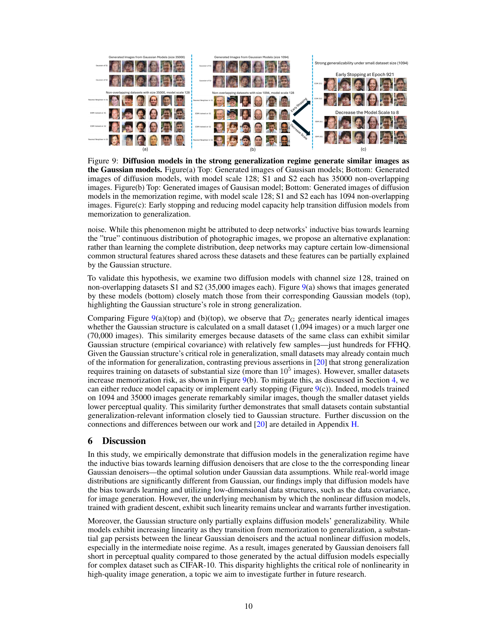
Model capacity significantly influences the generalizability of diffusion models. Smaller models, relative to the training dataset size, exhibit a strong inductive bias towards learning Gaussian structures. This bias is beneficial for generalization, allowing the model to capture fundamental data characteristics and produce high-quality samples beyond the training data. Larger, overparameterized models initially demonstrate this Gaussian bias during early training phases before transitioning to memorization. This highlights the importance of training duration and early stopping to harness this inductive bias while avoiding overfitting. The interplay between model capacity, training data size, and training duration is crucial in understanding how diffusion models achieve strong generalization, suggesting an optimal regime exists that balances model expressiveness with the avoidance of overfitting.
Linear Distillation#
The technique of “linear distillation” in the context of diffusion models involves approximating complex, non-linear diffusion denoisers with simpler linear models. This simplification facilitates a deeper understanding of the internal workings of diffusion models, particularly their generalization capabilities. By replacing the non-linear function mappings with linear counterparts, researchers aim to uncover the core properties that enable generalization beyond the training data. This approach is particularly insightful when examining how diffusion models capture and leverage the underlying Gaussian structure of the data distribution. The linear models offer a tractable way to analyze how the original model incorporates the training data’s empirical mean and covariance, revealing inductive biases that might otherwise be hidden within the complexities of non-linear networks. Linear distillation acts as a powerful tool to bridge the theoretical understanding of diffusion models with their empirical success, providing a clearer picture of why these models exhibit such strong generalization capabilities.
More visual insights#
More on figures

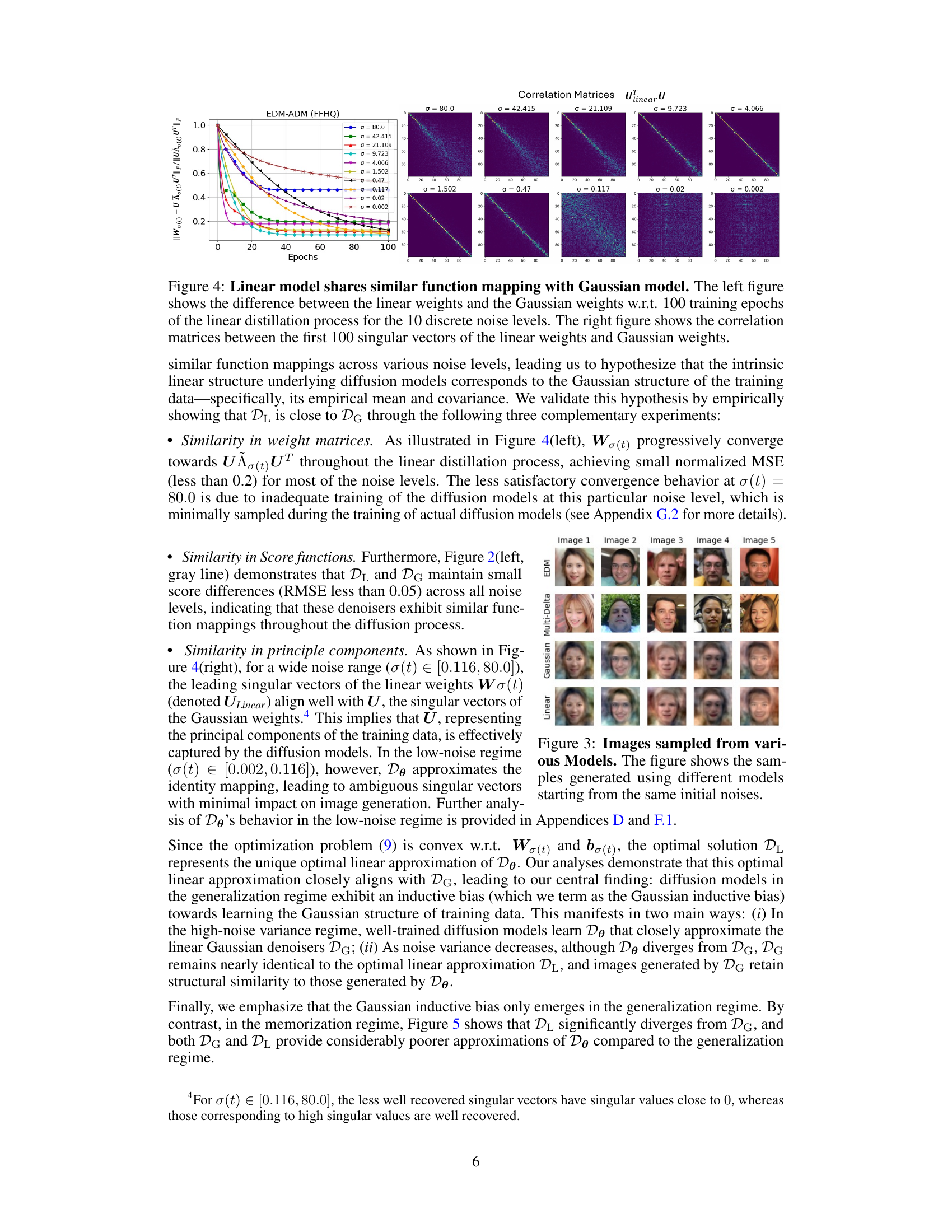
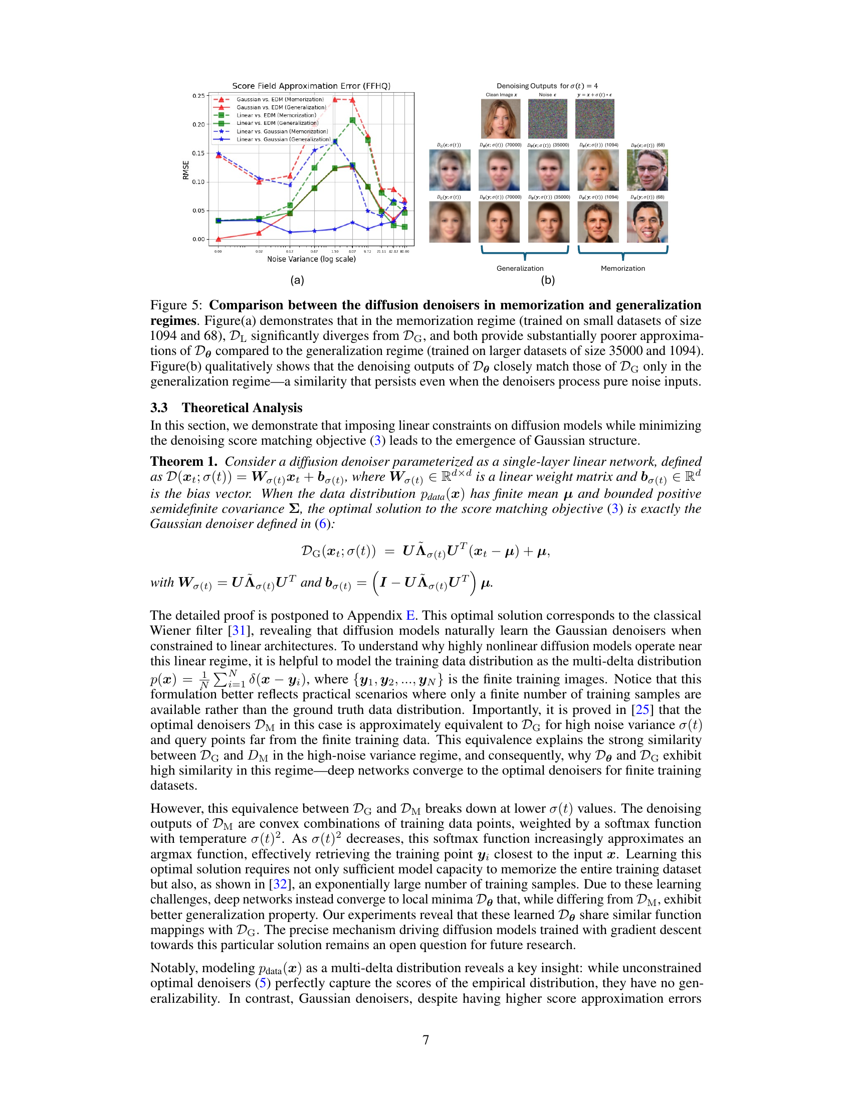
This figure shows a comparison of score functions and sampling trajectories for four different models: the actual diffusion model (EDM), a multi-delta model, a linear model, and a Gaussian model. The left panel plots the root mean square error (RMSE) between the score functions of each model and the actual diffusion model across different noise levels. The right panel displays the sampling trajectories, showing how each model generates samples starting from random noise. The close overlap between the linear and Gaussian model curves in the left panel indicates that they generate similar samples.

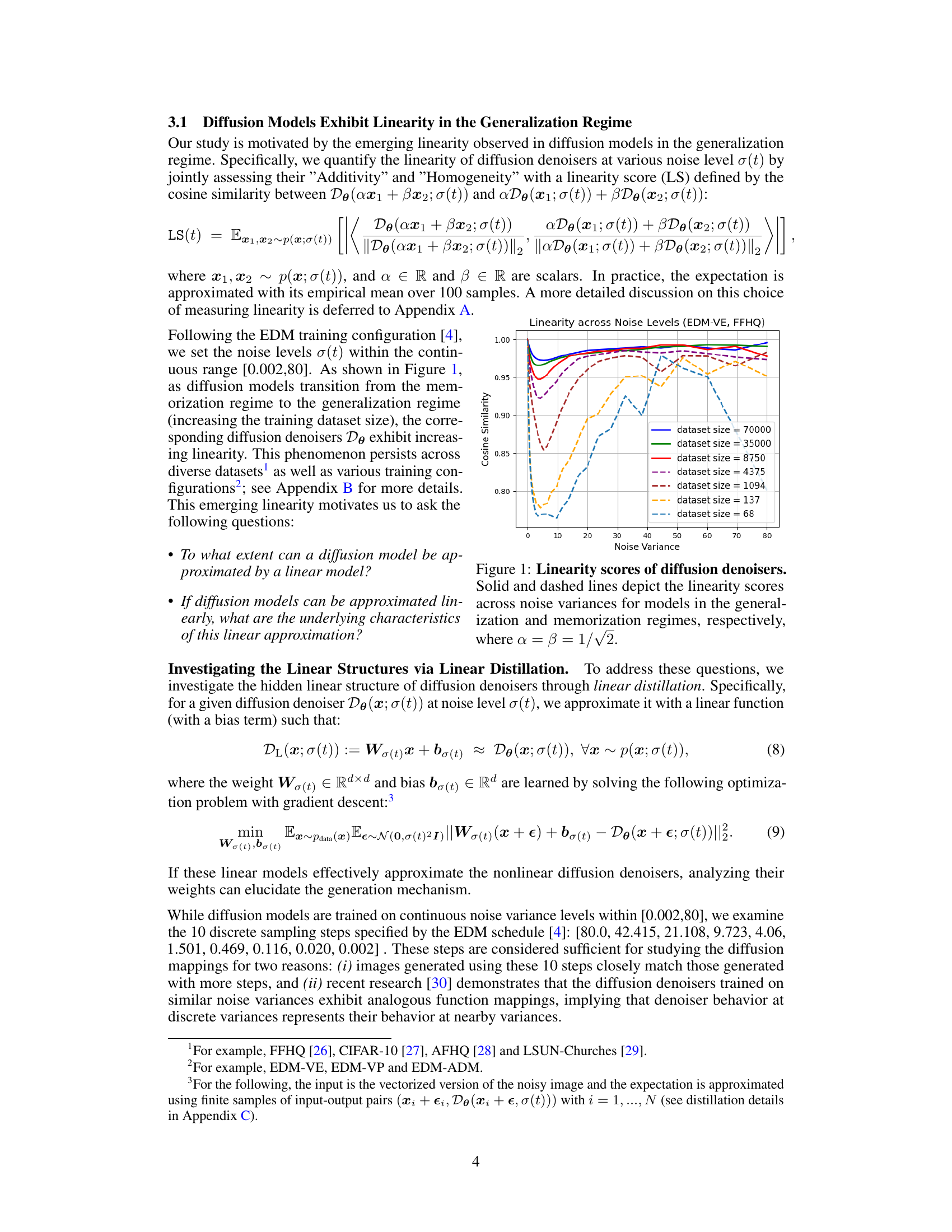
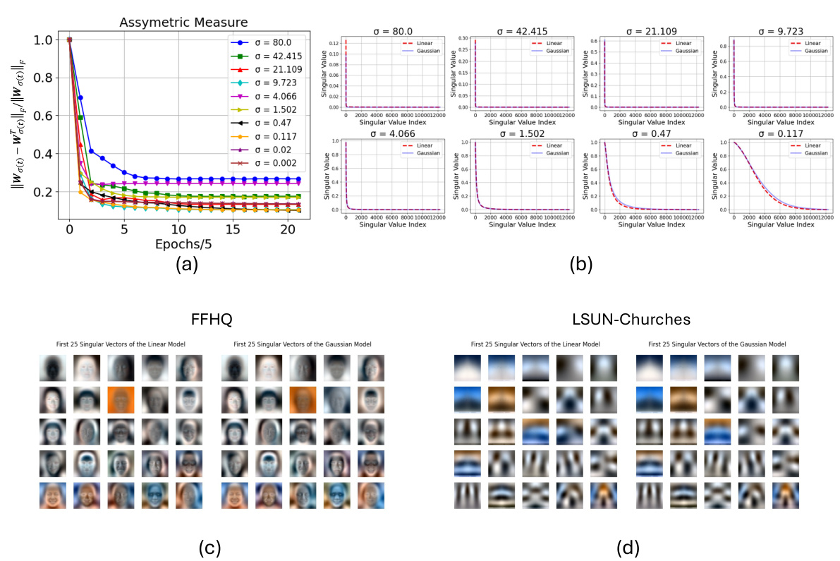
This figure shows two plots. The left plot shows how the weights of the linear model (trained to approximate diffusion denoisers) evolve over 100 training epochs and how they become increasingly similar to the weights of the Gaussian model (optimal denoiser for Gaussian data). The right plot visualizes the correlation between the principal components of the linear model and the Gaussian model for different noise levels. High correlation suggests that linear models effectively capture the Gaussian structure of the data.
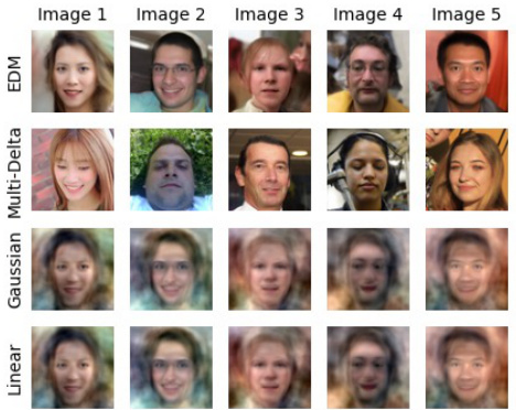
This figure compares the score approximation error and sampling trajectories of four different generative models: the actual diffusion model (EDM), a Multi-Delta model, a linear model, and a Gaussian model. The left panel shows that the linear model and the Gaussian model closely approximate the score function of the actual EDM, especially in intermediate noise levels. The right panel visually demonstrates the similarity between the sampling trajectories of the linear and Gaussian models, further reinforcing their close approximation to the actual diffusion model’s behavior.
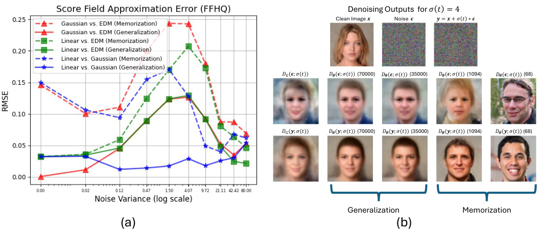
This figure shows a comparison of score field approximation errors and sampling trajectories for four different models: the actual diffusion model (EDM), a Multi-Delta model, a linear model, and a Gaussian model. The left panel displays the root mean square error (RMSE) between the score functions of each model and the actual diffusion model across various noise levels. The right panel illustrates the sampling trajectories—the sequence of images generated during the denoising process—for each model. The results indicate that the linear model’s score function closely approximates that of the Gaussian model, and both are relatively close to the actual diffusion model’s score function, especially at intermediate noise levels. This suggests that the linear and Gaussian models effectively capture the essential aspects of the actual diffusion model’s behavior.

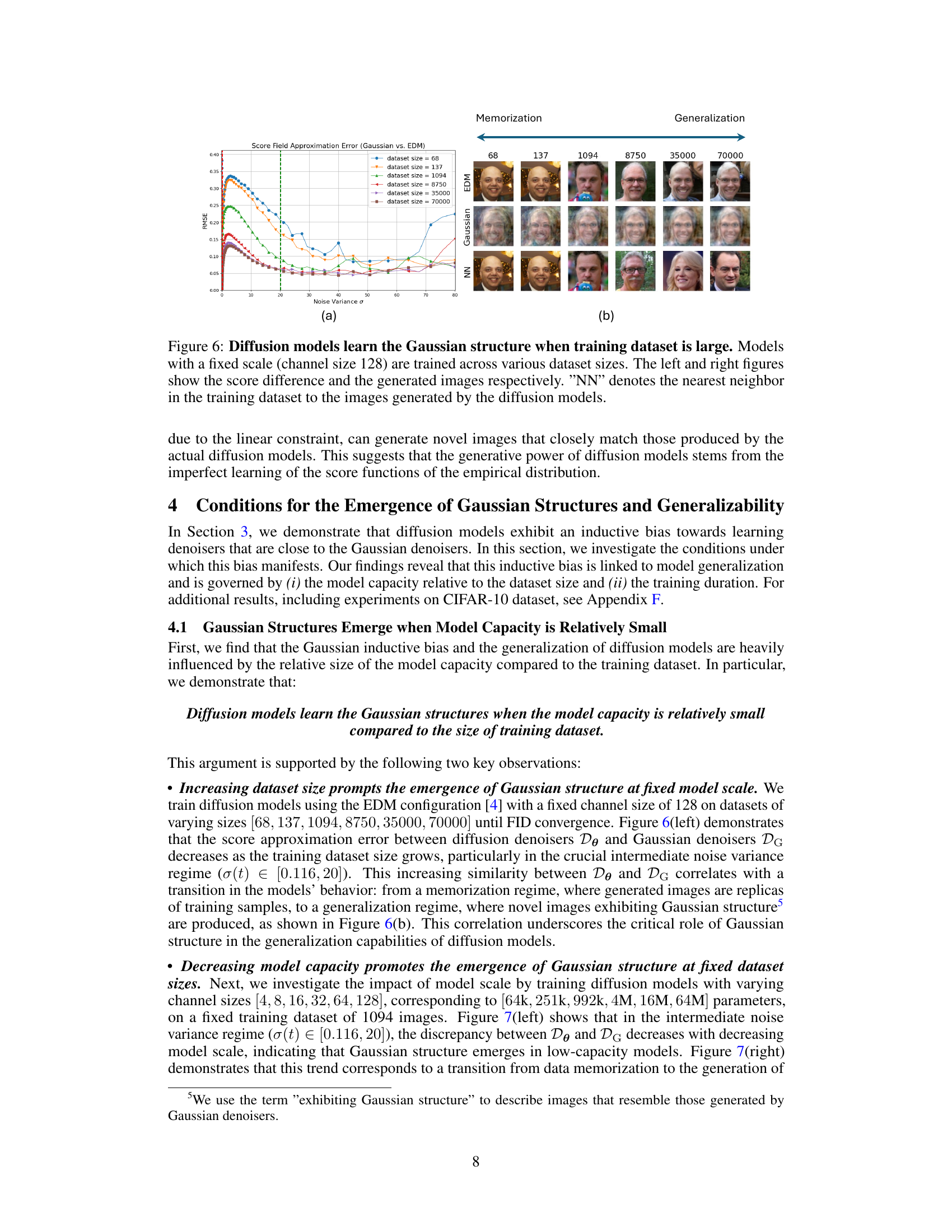
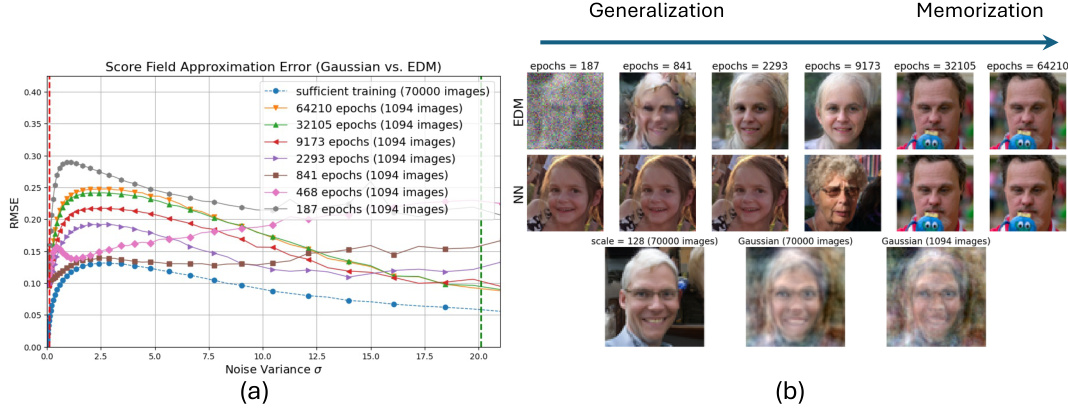
This figure shows the results of an experiment where diffusion models with a fixed capacity (128 channels) were trained on datasets of varying sizes (68, 137, 1094, 8750, 35000, 70000 images). The left panel plots the root mean square error (RMSE) between the score function of the trained model and the score function of a multivariate Gaussian distribution fitted to the training data, across different noise levels. The right panel shows generated images from the trained models, along with the nearest neighbor from the training set, and the images generated by the Gaussian model. The figure demonstrates that as the training dataset size increases, the RMSE decreases, indicating that the model learns the Gaussian structure of the data. This is further corroborated by the images which shows that as the training dataset increases, images generated by the diffusion model start to resemble those generated by the Gaussian model, rather than simple copies of the training data.

This figure shows that as the training dataset size increases, the score approximation error between the diffusion denoisers and the optimal Gaussian denoisers decreases, especially in the intermediate noise variance regime. The generated images transition from being simple replications of the training data to novel images that exhibit Gaussian structure. The results suggest that the Gaussian structure of the training data plays a critical role in the generalization capabilities of diffusion models.
This figure displays two subfigures. The left subfigure shows the score approximation error for four different models: EDM (Energy-based Diffusion Model), Multi-Delta, Linear, and Gaussian. The x-axis represents the noise variance, and the y-axis represents the Root Mean Square Error (RMSE). The plot highlights the close agreement between the linear and Gaussian model approximation errors, particularly in the mid-range noise variances. The right subfigure presents the sampling trajectories for each of the four models, demonstrating similar function mappings between the Linear and Gaussian models. These findings suggest that the function mappings of the effective generalized diffusion models can be well approximated by linear models that capture the Gaussian structures of the dataset.

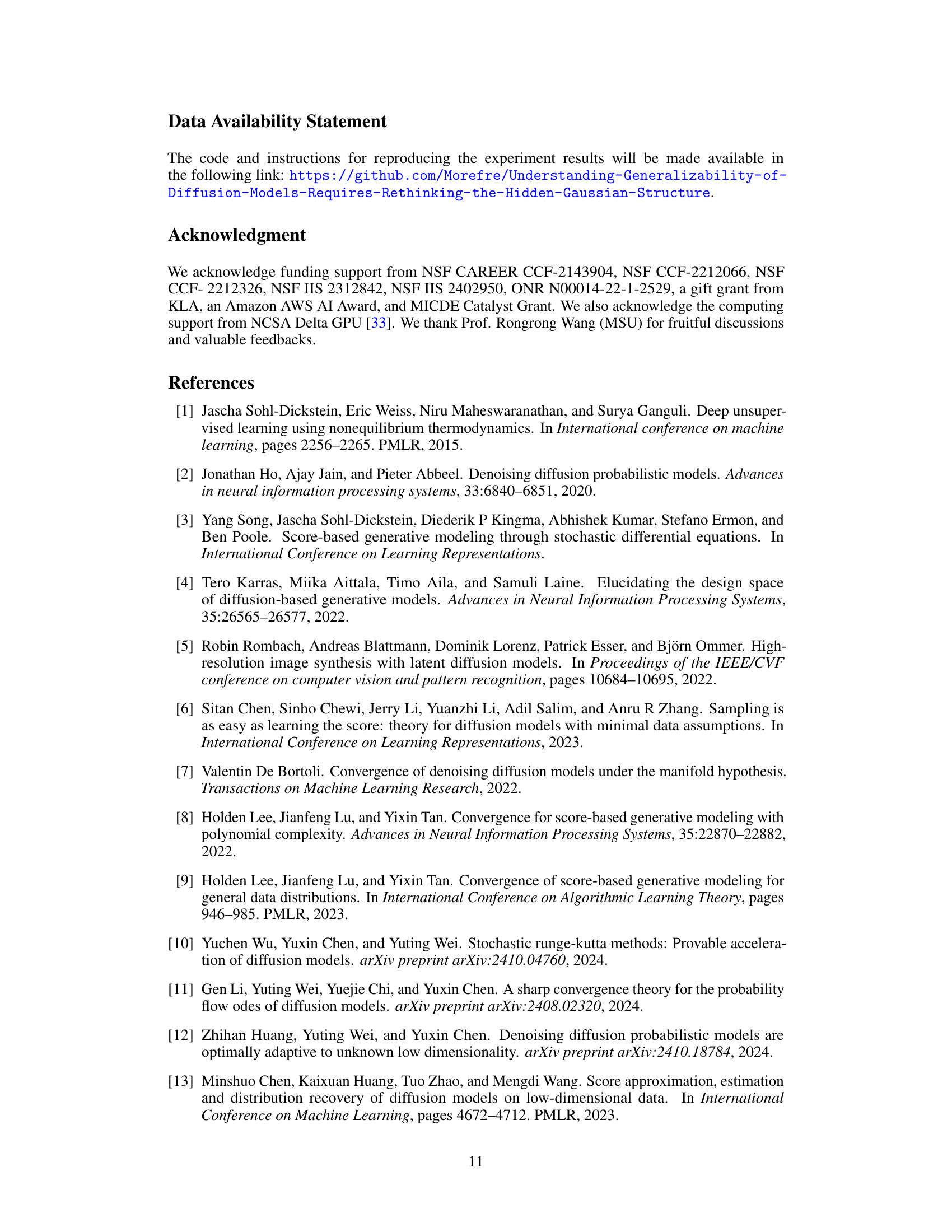
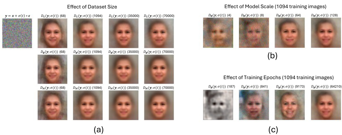
This figure demonstrates the strong generalization phenomenon observed in diffusion models. The top row shows images generated by Gaussian models trained on two separate, non-overlapping datasets (S1 and S2). The bottom row shows images generated by diffusion models trained on the same datasets. (a) shows that when trained on large datasets (35000 images), diffusion models generate images very similar to the Gaussian models. (b) shows that when trained on small datasets (1094 images), the diffusion model’s images are closer to those in the training set, demonstrating memorization. (c) Illustrates how early stopping or reducing model capacity can allow the diffusion model to transition from memorization to generalization, producing images more similar to the Gaussian models.

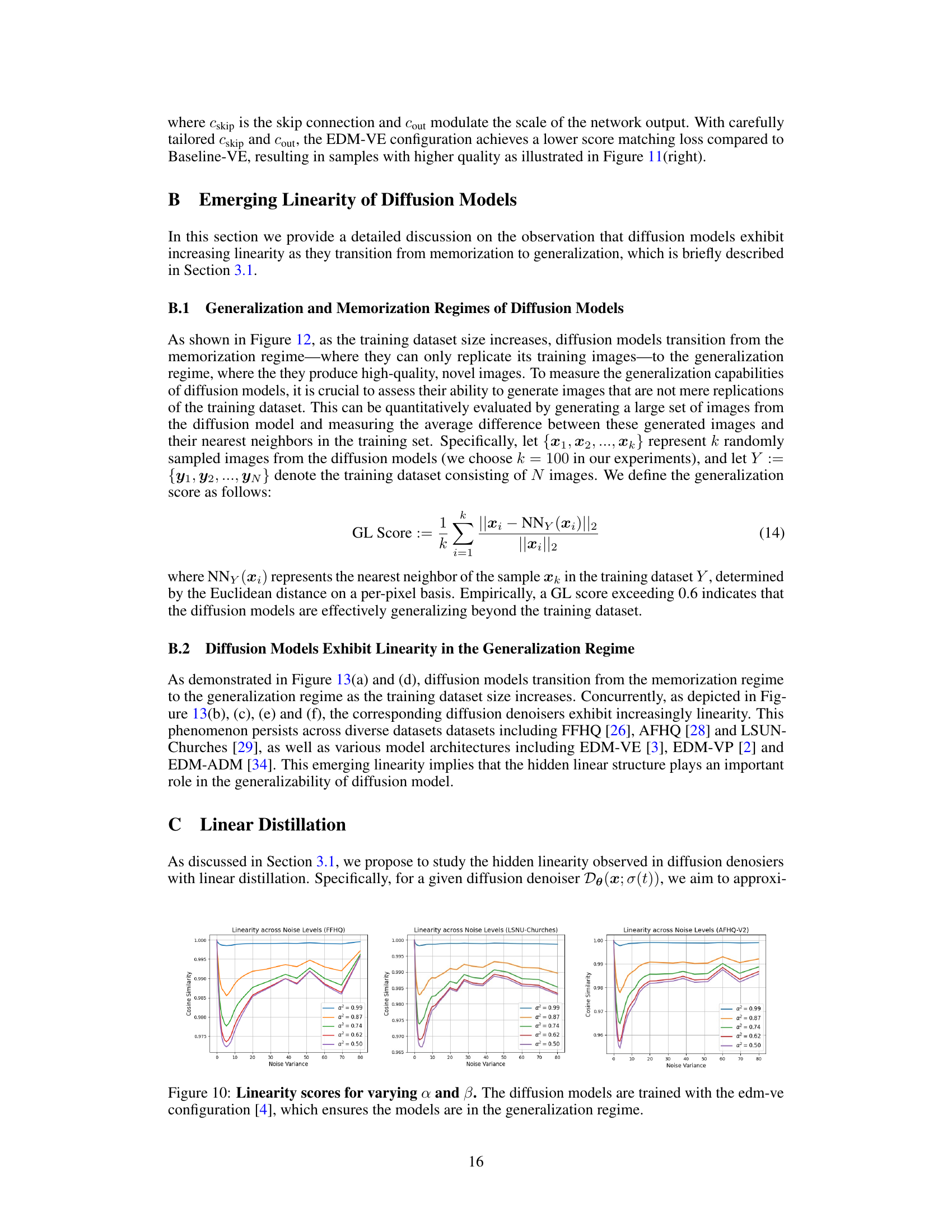
This figure shows the linearity scores for different values of α and β across different noise levels. The linearity score measures how well the diffusion denoisers satisfy additivity and homogeneity properties, indicating how close the denoisers are to linear functions. The x-axis represents noise variance, while the y-axis represents the cosine similarity between the actual output of the denoiser and the expected output based on linear behavior. The different lines correspond to different values of α and β (used to calculate the input for the linearity score). The EDM-VE configuration is used to train the models, ensuring they operate in the generalization regime.

This figure shows a comparison of linearity scores and sampling trajectories for different models. The left panel displays the linearity scores across different noise levels for EDM-VE (a well-trained diffusion model), Baseline-VE (a less well-trained diffusion model), a linear model, and a Gaussian model. The right panel illustrates the generation trajectories of these same models, showing how they progressively denoise a random noise vector into a clean image. This helps to visualize how linearity affects the models’ image generation process.

This figure shows how the generalization ability of diffusion models changes as the training dataset size increases. With small datasets, the models reproduce training images (memorization). As the dataset size increases, the models generate novel images beyond the training set (generalization). This is demonstrated using both FFHQ and CIFAR-10 datasets.
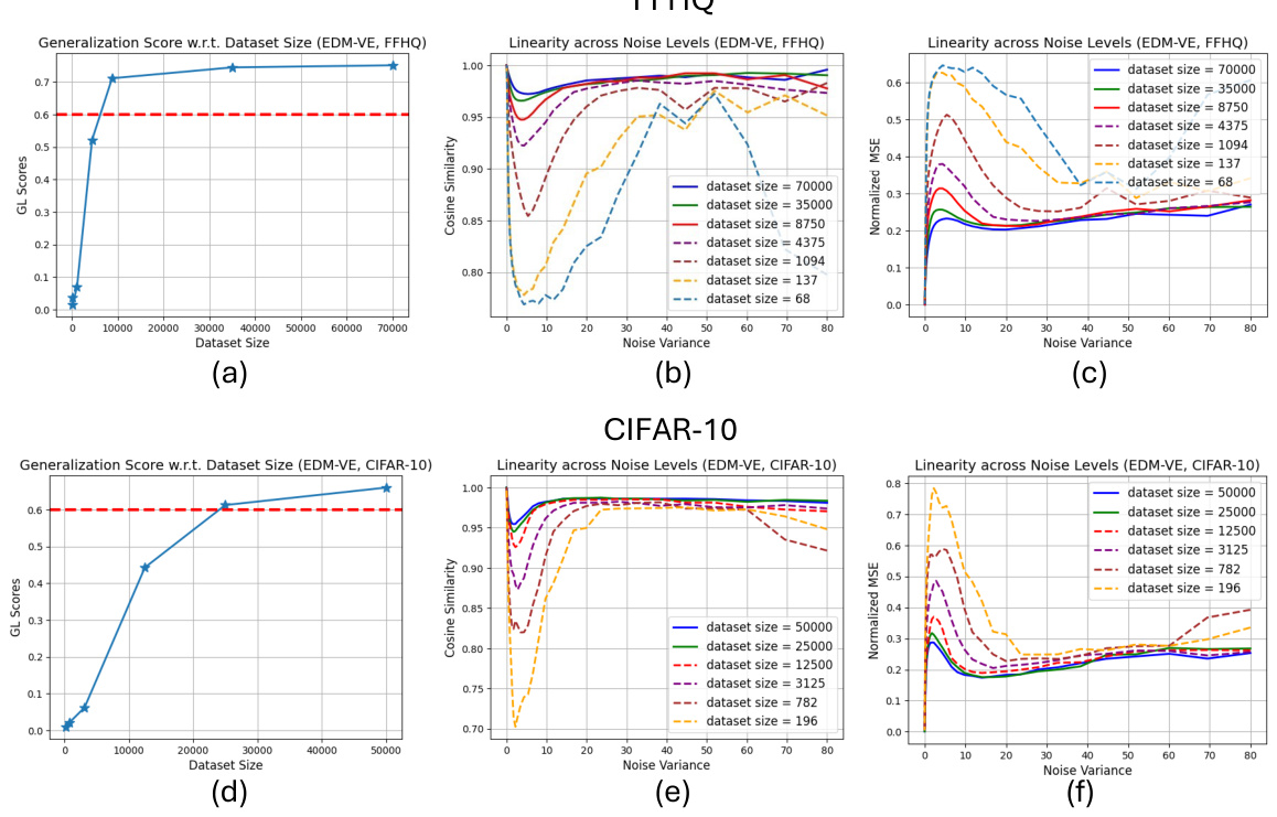
This figure shows the linearity scores of diffusion denoisers across different noise levels for models trained in both the generalization and memorization regimes. The linearity score measures how closely the denoiser’s output approximates a linear function of the input. The solid lines represent models in the generalization regime (trained on larger datasets), and the dashed lines represent models in the memorization regime (trained on smaller datasets). The x-axis represents noise variance, and the y-axis represents the linearity score. The plot demonstrates that as the training dataset size increases (moving from memorization to generalization), the linearity of the diffusion denoiser increases across all noise variance levels.
This figure shows the linearity scores of diffusion denoisers across different noise levels for models trained in both generalization and memorization regimes. The linearity score measures how close the denoisers are to being linear functions. The solid lines represent models in the generalization regime (producing novel images), while the dashed lines represent models in the memorization regime (primarily reproducing training data). The plot demonstrates that as models transition from memorization to generalization, their linearity increases.

This figure shows the difference between the output of the diffusion models and the input for various noise levels. The difference is measured using normalized MSE and cosine similarity. The results show that the difference quickly approaches zero in the low-noise variance regime, regardless of model architecture.

This figure shows a comparison of score approximation errors and sampling trajectories for four different models: the actual diffusion model (EDM), the multi-delta model, a linear model, and a Gaussian model. The left panel displays the root mean squared error (RMSE) between the score functions of each model and the actual diffusion model across various noise levels. The right panel shows the sampling trajectories of the different models, which are visualizations of how the models gradually transform random noise into an image. Notably, the Gaussian model’s curve closely matches the linear model’s curve, indicating the similarity between their function mappings.
This figure shows a comparison of score approximation errors and sampling trajectories for different models. The left plot displays the root mean square error (RMSE) between the score functions of various models (actual diffusion model, multi-delta model, linear model, and Gaussian model) and the actual diffusion model’s score function, across various noise levels. The right plot shows the image generation trajectories of the four models, starting from the same random noise. The close overlap between the curves for the linear and Gaussian models indicates that these two models have very similar function mappings, suggesting the learned score functions have a hidden Gaussian structure.

This figure shows a comparison of the score approximation error and sampling trajectories for four different models: the actual diffusion model (EDM), a multi-delta model, a linear model, and a Gaussian model. The left panel displays the root mean squared error (RMSE) between the score functions of each model and the actual diffusion model’s score function across different noise levels. The right panel shows the sampling trajectories – sequences of images generated during the denoising process – for each model. The key observation is that the Gaussian model closely matches the linear model, indicating that the linear model captures essential aspects of the diffusion process.

This figure shows the relationship between dataset size and the tendency for diffusion models to learn Gaussian structures. The left graph shows that as dataset size increases, the error between the score function of the actual diffusion model and the optimal Gaussian score decreases, indicating that larger datasets lead diffusion models to lean towards learning Gaussian-like distributions. The right side of the figure displays generated images from different models (actual diffusion model, Gaussian model, nearest neighbor model) and training dataset sizes, illustrating that larger datasets lead to generated images which closely resemble those generated by a Gaussian model, demonstrating better generalization.

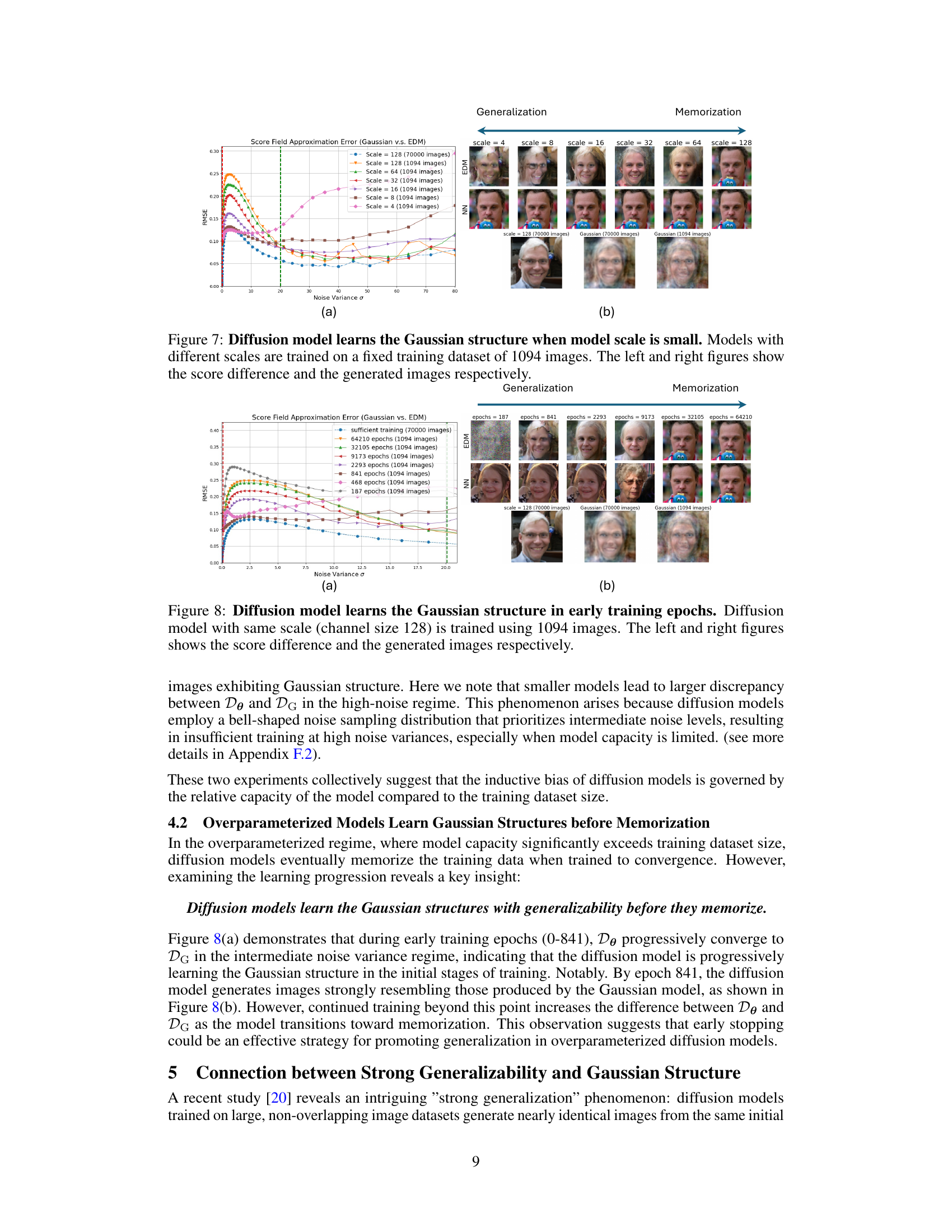
This figure shows the effect of model capacity on the learning of Gaussian structures in diffusion models. It demonstrates that when the model capacity (measured by the number of channels) is relatively small compared to the size of the training dataset, diffusion models exhibit an inductive bias towards learning Gaussian structures, leading to better generalization. The left panel shows the RMSE between the score functions of the diffusion model and the Gaussian model, while the right panel illustrates the generated images for models with different scales. This inductive bias is less pronounced when the model has larger capacity, leading to memorization of the training data.

This figure shows the relationship between training dataset size and the inductive bias of diffusion models towards learning Gaussian structures. The left graph shows that as the dataset size increases, the score approximation error between diffusion denoisers and Gaussian denoisers decreases, especially in the intermediate noise variance regime. This is visually confirmed by the right-hand side of the figure, which demonstrates that as dataset size increases, the generated images increasingly resemble those produced by Gaussian denoisers, moving from memorization of the training data to generalization. The ‘NN’ (nearest neighbor) images show that smaller datasets result in images very similar to the training set, while larger datasets produce more novel, realistic images.

This figure shows the results of training linear models to approximate the non-linear diffusion denoisers from diffusion models. The x-axis represents the training epochs, and the y-axis shows the normalized mean squared error (NMSE) between the weights of the linear model and the weights of the Gaussian model (the optimal linear model). Three different diffusion model architectures are shown: EDM-VE, EDM-ADM, and EDM-VP. The figure demonstrates that across different diffusion model architectures, the linear models converge towards the optimal Gaussian model, supporting the finding that diffusion models exhibit a bias towards learning Gaussian structures.

This figure compares the generated images from different diffusion models with varying network architectures (EDM-VE, EDM-VP, and EDM-ADM) and their corresponding Gaussian models. The comparison shows the similarities and differences between the images generated by the diffusion models and the images generated by approximating the data distribution with a multivariate Gaussian distribution. This highlights the inductive bias of diffusion models towards capturing and utilizing the Gaussian structure of the training dataset for image generation.

This figure presents a comparison of score field approximation error and sampling trajectories across four different models: the actual diffusion model (EDM), a Multi-Delta model, a linear model, and a Gaussian model. The left panel shows the root mean squared error (RMSE) between the score functions of each model and the actual diffusion model at various noise levels. The right panel displays the sampling trajectories, illustrating the evolution of generated samples as each model progresses through the reverse diffusion process. A key observation is that the Gaussian model’s trajectory closely resembles that of the linear model, supporting the idea that the Gaussian structure is a significant factor in the functionality of diffusion models.

This figure shows a comparison of score approximation errors and sampling trajectories for four different models: the actual diffusion model (EDM), a Multi-Delta model, a linear model, and a Gaussian model. The left panel plots the root mean squared error (RMSE) between the score functions of each model and the actual diffusion model, as a function of noise variance. The right panel shows image generation trajectories (i.e., the sequence of images generated during the denoising process) for each model. The results highlight a strong similarity between the linear model and Gaussian model, indicating that the learned score functions of diffusion models in the generalization regime are close to being optimal for a multivariate Gaussian distribution.

This figure demonstrates the strong generalization phenomenon observed in diffusion models. The top row shows images generated by Gaussian models trained on two non-overlapping datasets (S1 and S2) of different sizes (35,000 and 1,094 images). The bottom row shows corresponding images from diffusion models trained on the same datasets and model scale 128. In (a), with larger datasets, the diffusion models generalize well producing similar images to the Gaussian models. In (b), with smaller datasets, the diffusion models only reproduce images from the training dataset (memorization), showcasing the difference. (c) provides a strategy to mitigate the memorization effect by using early stopping or reducing the model capacity.
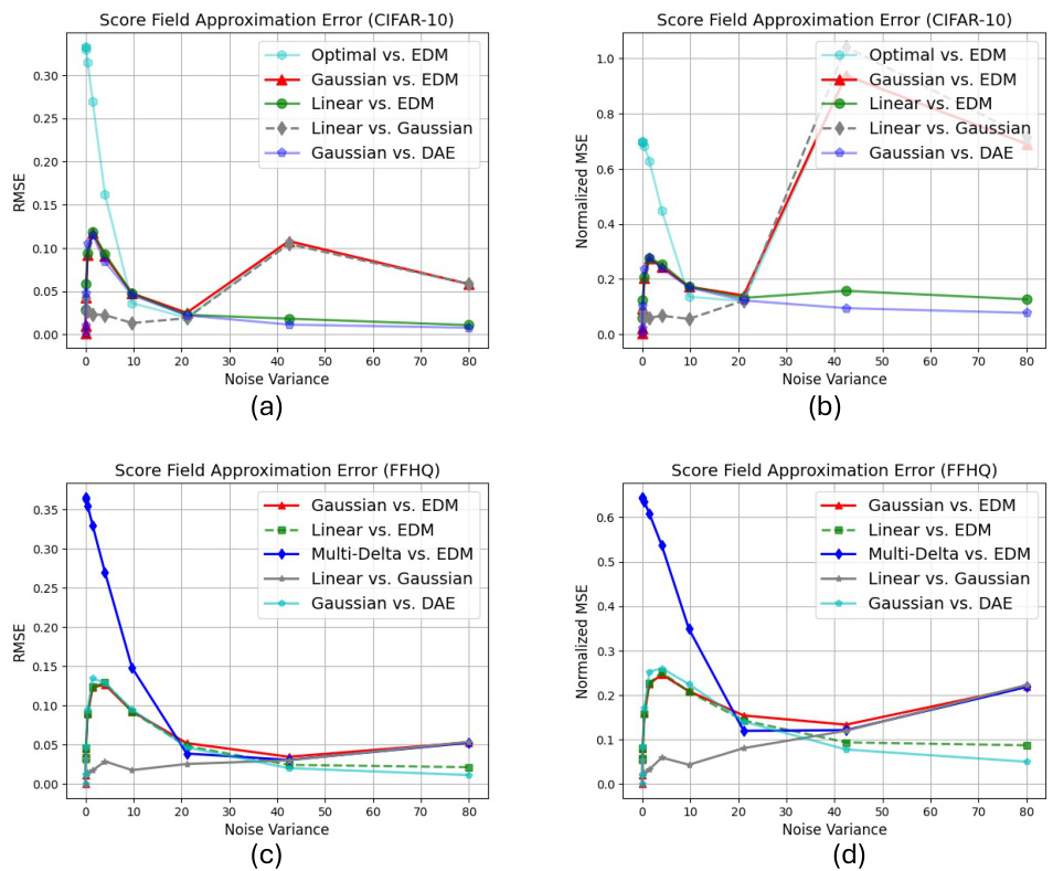
This figure shows a comparison of score approximation errors and sampling trajectories for four different models: the actual diffusion model (EDM), a Multi-Delta model, a linear model, and a Gaussian model. The left panel displays the root mean squared error (RMSE) between the score functions of each model and the actual diffusion model across different noise variance levels. The right panel illustrates the sampling trajectories of the four models, starting from random Gaussian noise and progressing through denoising steps until a final image is generated. The close overlap between the linear and Gaussian model curves suggests similar function mappings.

This figure shows the linearity scores of diffusion denoisers across different noise levels for models trained in both the generalization and memorization regimes. The linearity score measures how close the denoiser’s behavior is to a linear function. The results indicate that diffusion models in the generalization regime exhibit a greater degree of linearity, suggesting that linearity is a key aspect of their generalizability.

The figure shows linearity scores of diffusion denoisers across different noise levels for models trained in both generalization and memorization regimes. The linearity score measures how close a denoiser’s output is to a linear combination of its inputs. The solid lines represent models in the generalization regime, showing increasing linearity as dataset size increases, and the dashed lines represent models in the memorization regime, exhibiting lower linearity. The parameter α=β=1/√2 controls the weighting of two inputs when calculating the linearity score.

This figure shows the effects of perturbing the input image along the first singular vector of the Jacobian matrix at different noise levels. In the high-noise regime, this leads to major changes in the generated image (e.g., changing the class of the image). In the intermediate-noise regime, there are changes to details, but the overall structure remains similar. Finally, in the low-noise regime, the perturbation has little to no effect on the output image.
Full paper#

