↗ OpenReview ↗ NeurIPS Homepage ↗ Chat
TL;DR#
Many machine learning models struggle with missing data, especially when interpretability is crucial. Simply imputing missing values or using many indicator variables can complicate models and reduce their interpretability. This paper addresses these issues by proposing a novel approach.
The proposed solution is M-GAM, a sparse generalized additive model. Unlike methods that impute missing data or add many indicator variables, M-GAM directly incorporates missingness indicators and their interactions while maintaining sparsity using l0 regularization. Experiments demonstrate that M-GAM offers comparable or superior performance to existing methods but with significantly improved sparsity and reduced computation time.
Key Takeaways#
Why does it matter?#
This paper is crucial for researchers working with interpretable models and handling missing data. It introduces a novel model (M-GAM) that directly incorporates missingness into the model’s reasoning, offering superior accuracy and sparsity compared to imputation methods. This opens avenues for improving interpretability in various machine learning applications where missing data is a common challenge. The focus on sparsity addresses overfitting issues often faced when using missingness indicators, making M-GAM highly relevant to current research on interpretable and efficient machine learning.
Visual Insights#
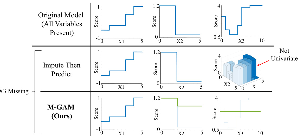
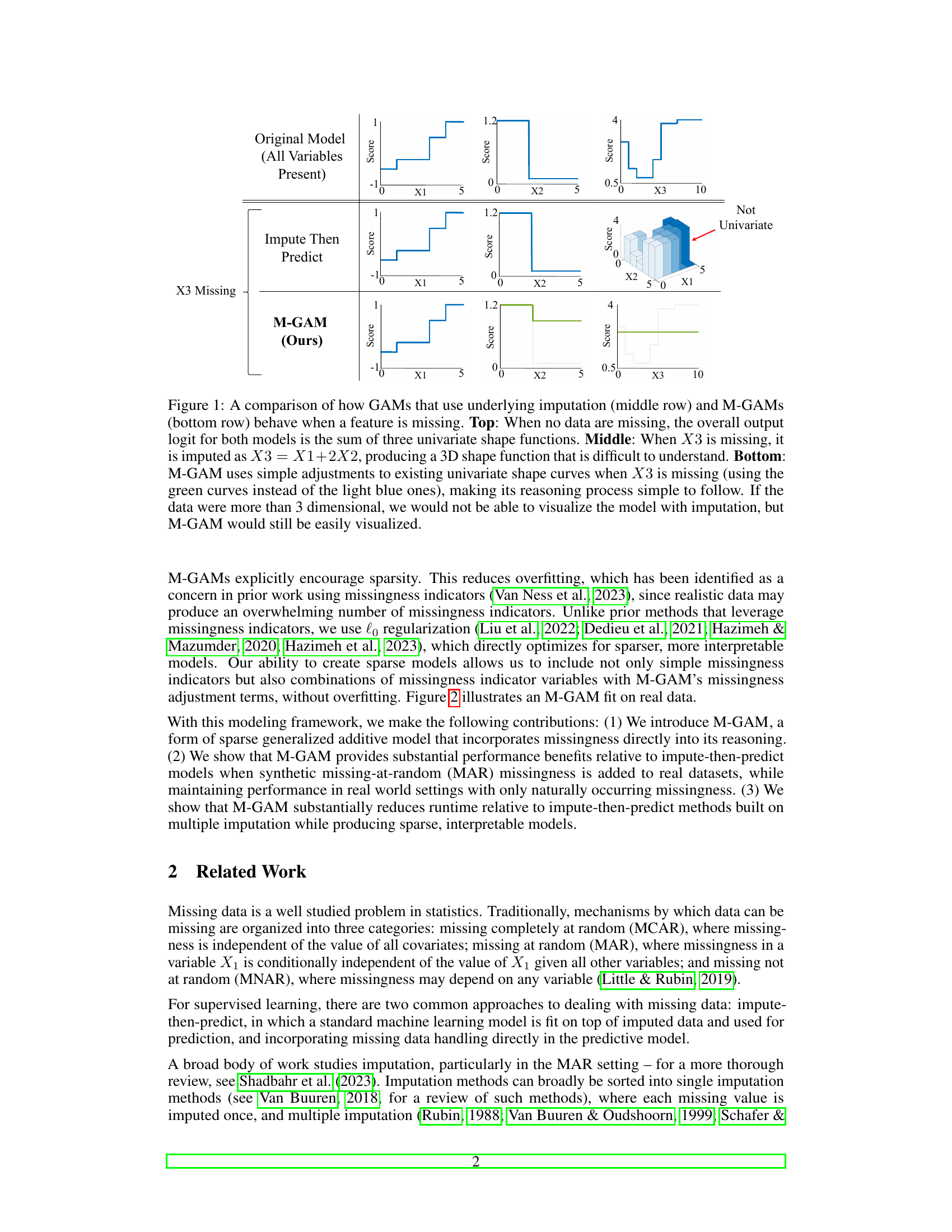
This figure compares the behavior of GAMs using imputation versus M-GAM when a feature is missing. The top row shows a standard GAM with all features present. The middle row illustrates that imputing missing values (e.g., using X3 = X1 + 2X2) creates complex, non-univariate interactions making interpretation difficult. The bottom row demonstrates M-GAM’s approach: using simple adjustments to existing univariate curves. This preserves interpretability, even with higher-dimensional data, where imputation would be highly complex.

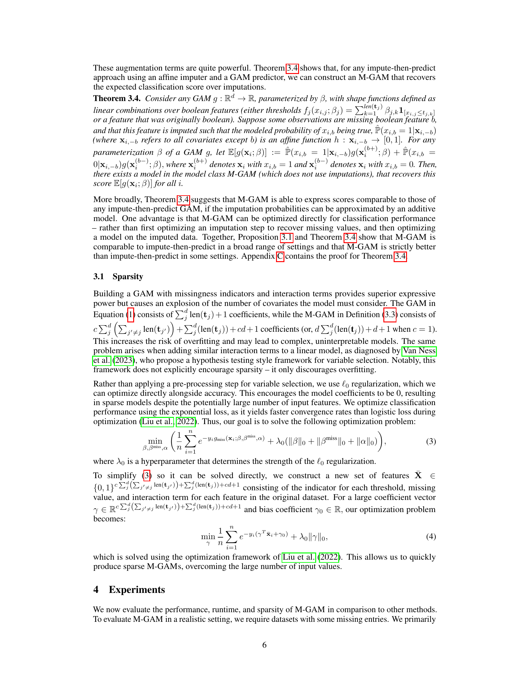
This table shows the conditional probability of a variable (X1) being missing given the values of another variable (X2) and the outcome (Y). It defines the mechanism for introducing synthetic missingness into the data in a way that is Missing at Random (MAR). The probability of missingness depends on the outcome (Y) and X2. If X2 is above the 60th percentile, then the probability of X1 being missing is ‘r’ if Y = 1 and 0 if Y = 0. If X2 is below the 60th percentile, the opposite is true. This creates a dependence between the outcome and the probability of missingness, making it MAR, but not MCAR.
In-depth insights#
Interpretable GAMs#
Interpretable Generalized Additive Models (GAMs) offer a powerful approach to modeling complex relationships in data while maintaining interpretability. Their additive structure, where the overall prediction is a sum of individual effects from each predictor variable, makes them inherently transparent. However, traditional GAMs struggle with missing data, often necessitating imputation techniques that obscure the model’s interpretability. This is where the focus on interpretable GAMs becomes crucial. By incorporating handling of missing values directly into the GAM framework, rather than relying on pre-processing steps like imputation, we can preserve both the model’s accuracy and its transparency. The development of methods that directly model the influence of missingness on the additive functions is a key advance, preventing the introduction of complex interactions that would obscure the model’s interpretability and potentially lead to overfitting. This is a significant step toward creating reliable and easily-understood models, especially in domains where transparency is paramount, such as healthcare or finance. Achieving sparsity in these models through methods like L0 regularization is essential to prevent overfitting and maintain the model’s interpretability by limiting the number of terms that significantly contribute to the prediction. The focus on interpretable GAMs is timely and essential, addressing a significant limitation of traditional GAMs in the context of real-world datasets with missing values.
M-GAM Approach#
The M-GAM approach presents a novel method for handling missing data in generalized additive models (GAMs) while preserving interpretability. Instead of imputation, which can complicate model interpretation and introduce bias, M-GAM directly incorporates missingness indicators and interaction terms into the model. This allows for the explicit modeling of how missingness influences the relationship between features and the outcome. The use of L0 regularization is crucial for maintaining model sparsity and interpretability, preventing overfitting. This is particularly important when dealing with missing data because including missingness indicators alone can lead to an explosion of the number of parameters. M-GAM demonstrates superior performance compared to various impute-then-predict models, especially in situations with informative missingness where the missingness pattern itself carries predictive value. The model’s superior runtime performance and its ability to produce interpretable results are significant advantages in many applications where interpretability is highly valued.
MAR Handling#
The research paper’s approach to handling Missing At Random (MAR) data is a key strength. Instead of imputation, which can introduce complexities and hinder interpretability, the method directly incorporates missingness indicators and interaction terms into a sparse Generalized Additive Model (GAM). This innovative technique allows the model to learn the relationships between features and the target variable while explicitly acknowledging and leveraging the information present in the missing data patterns. The use of L0 regularization is crucial for maintaining sparsity and interpretability, preventing overfitting often associated with high-dimensional models incorporating missingness indicators. The results demonstrate that this strategy achieves comparable or superior performance compared to imputation-based methods, while significantly improving sparsity and maintaining the model’s interpretability. This addresses a critical limitation in many MAR handling approaches which sacrifice interpretability for the sake of accuracy. The approach’s focus on retaining model interpretability and sparsity is particularly valuable in high-stakes applications, such as those mentioned in the paper, where understanding the model’s decision-making process is paramount. Overall, the method presents a significant advancement in effectively and transparently handling MAR data.
Sparsity Benefits#
The concept of sparsity, crucial in machine learning, especially for interpretable models, is central to the paper’s contribution. Sparsity directly improves interpretability by reducing the number of model parameters and their interactions. The authors address the challenge of missing data, which often leads to dense models with an explosion of indicator variables representing missingness. By leveraging L0 regularization, M-GAM achieves sparsity while handling missing data effectively. This is a significant advantage over traditional imputation methods which tend to create dense, complex models hindering interpretability. The paper highlights that M-GAM’s sparsity leads to superior performance compared to other methods, particularly in scenarios with informative missingness, where the missingness itself carries valuable predictive information. Balancing sparsity and accuracy is a key strength of the proposed M-GAM framework.
Future Work#
The research paper’s ‘Future Work’ section could explore several promising avenues. Extending M-GAM’s applicability to various data types beyond binary classification is crucial. Investigating its performance with continuous, multi-class, or other structured data would broaden its impact. Developing more sophisticated regularization techniques is essential. While L0 regularization promotes sparsity, exploring alternative methods might yield even better interpretability and performance. Addressing potential biases and distribution shifts in missing data is critical. The current model assumes missing data is Missing At Random; investigating scenarios with non-random missingness and handling bias in the data is vital. Finally, integrating uncertainty quantification directly into the M-GAM framework would enhance its reliability and interpretability, allowing the model to express uncertainty in its predictions effectively. All of these future directions represent opportunities to improve model accuracy, efficiency, and robustness.
More visual insights#
More on figures
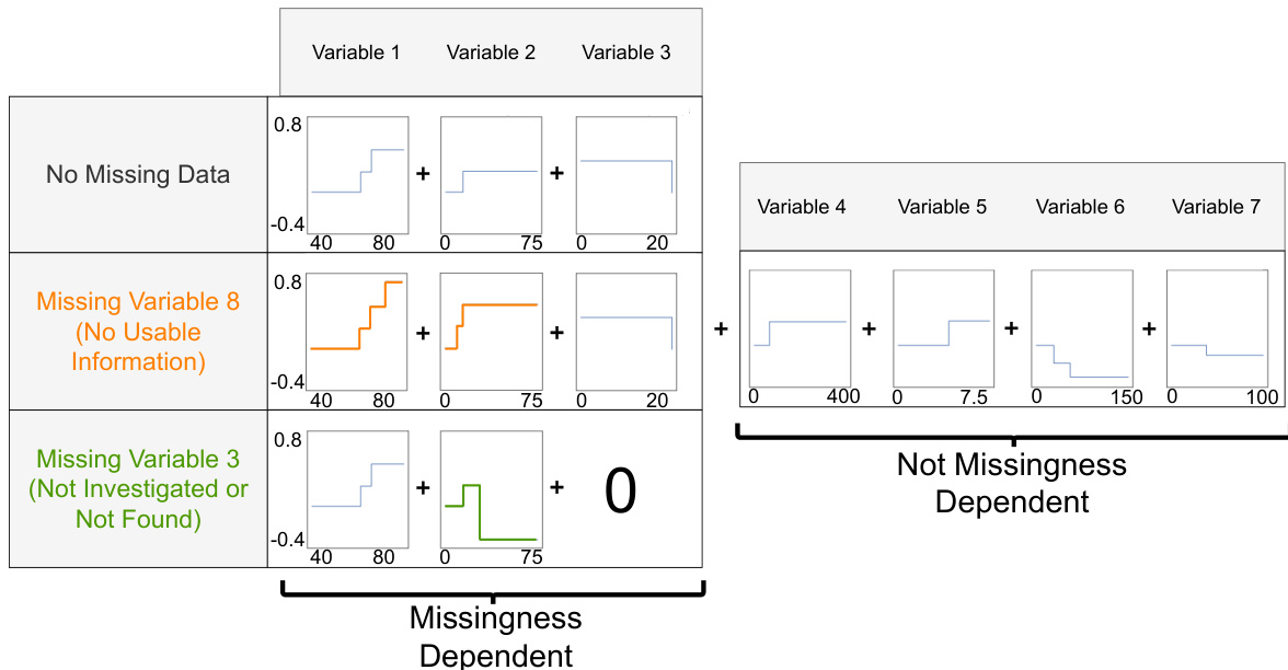
This figure demonstrates a generalized additive model (GAM) that incorporates missing data. It shows how the model adjusts its shape functions for features when other features have missing values, maintaining interpretability. The model uses additional boolean variables to indicate missingness and adjust shape curves accordingly. It achieves comparable performance to more complex models while improving interpretability and sparsity.

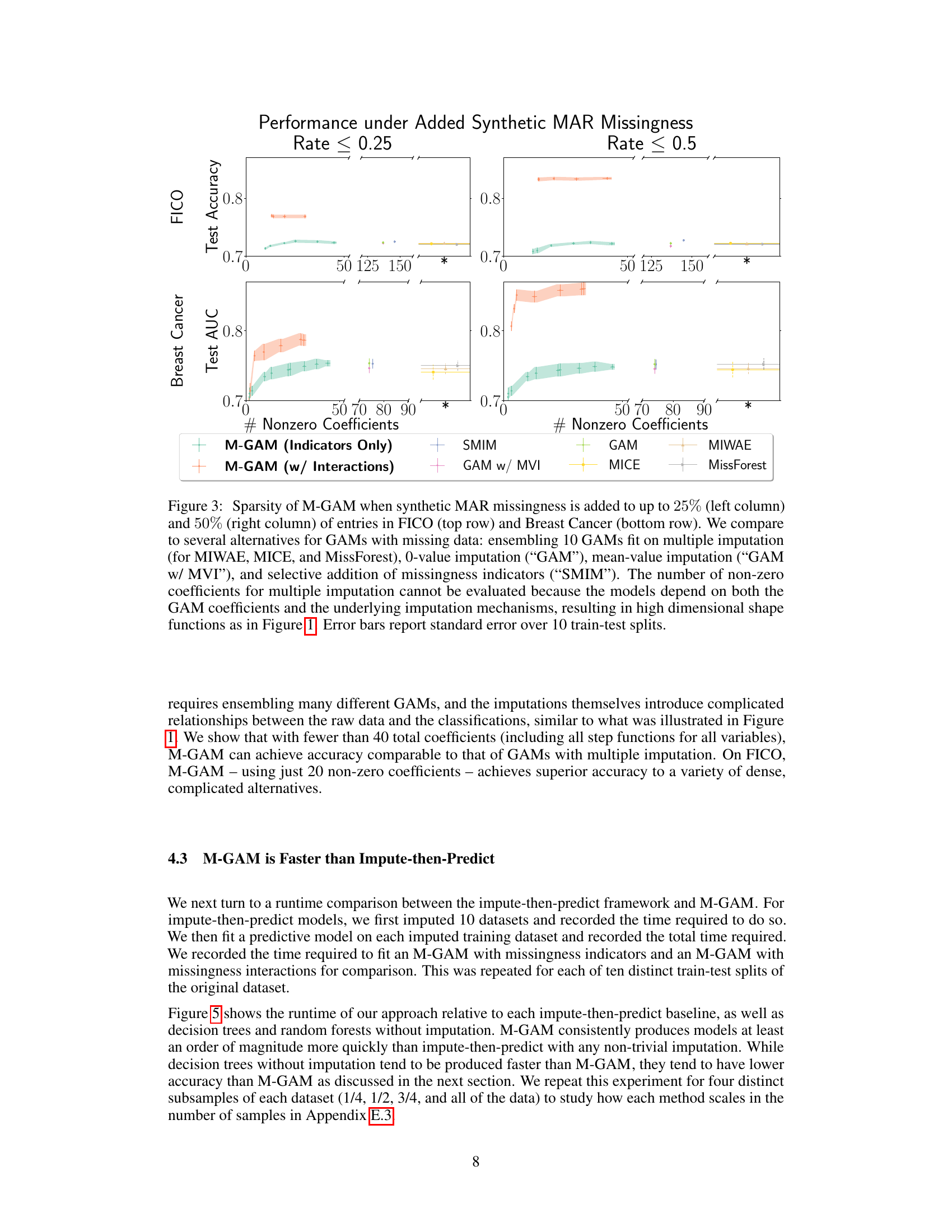
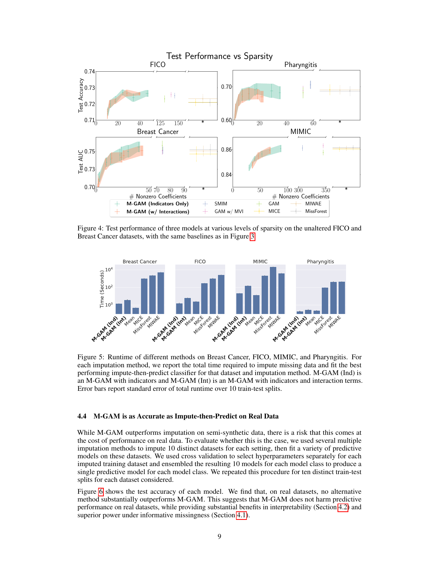
This figure compares the sparsity (number of non-zero coefficients) and test performance (accuracy or AUC) of M-GAM against several other methods for handling missing data in GAMs. It shows the impact of adding synthetic MAR missingness at different rates (25% and 50%) on two datasets (FICO and Breast Cancer). The comparison methods include multiple imputation techniques (MIWAE, MICE, MissForest), simple imputation methods (0-value, mean-value), and a method selectively adding missingness indicators (SMIM). The results highlight M-GAM’s ability to maintain sparsity and achieve comparable or better performance compared to other approaches, especially when dealing with higher rates of missing data. Error bars represent the standard error over 10 train-test splits.

This figure compares the sparsity (number of non-zero coefficients) and accuracy of M-GAM with other methods for handling missing data in two datasets (FICO and Breast Cancer) under different rates of synthetic MAR missingness. It shows that M-GAM achieves high accuracy with significantly fewer coefficients compared to methods that use imputation or simply add missingness indicators. The inability to evaluate non-zero coefficients for multiple imputation methods is highlighted due to the increased model complexity introduced by the imputation process.

The figure compares the sparsity (number of non-zero coefficients) and test performance (accuracy or AUC) of M-GAM with other methods for handling missing data in two datasets (FICO and Breast Cancer). Synthetic missing data at different rates (25% and 50%) were added to evaluate performance. The other methods include multiple imputation techniques (MICE, MIWAE, MissForest) and a simple GAM model (with and without imputation). The results show that M-GAM achieves comparable or better accuracy with significantly fewer non-zero coefficients, demonstrating its superior sparsity.
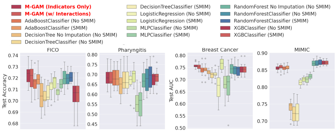
This figure compares the sparsity (number of non-zero coefficients) and test performance (accuracy or AUC) of M-GAM with different methods for handling missing data in the FICO and Breast Cancer datasets. Synthetic MAR missingness was added at rates of up to 25% and 50%. The results show that M-GAM achieves comparable or better accuracy than other methods while maintaining significantly greater sparsity, especially when compared with imputation-based methods that have high dimensional shape functions.

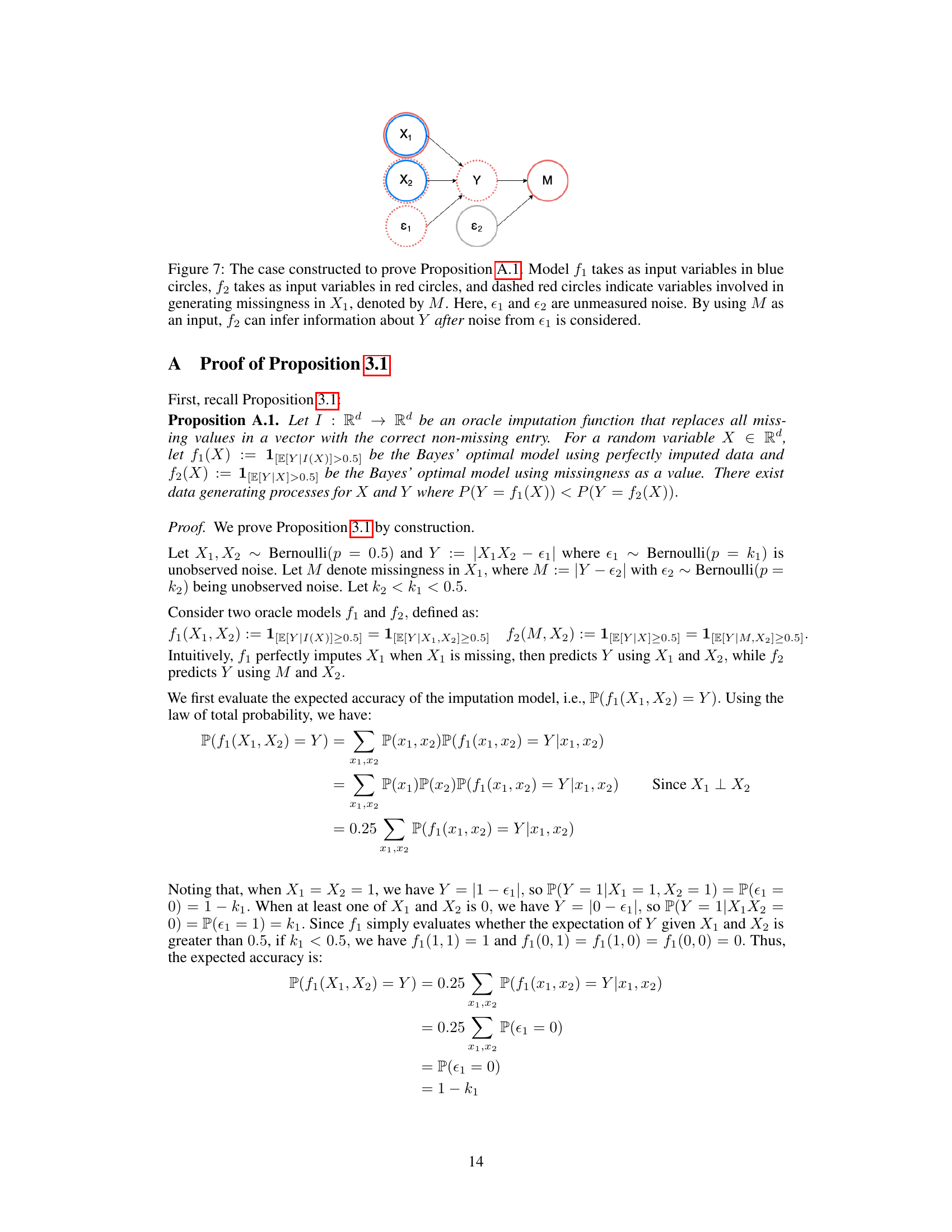
This figure presents a Bayesian network illustrating the relationship between variables in a constructed example used to prove Proposition 3.1. The proposition demonstrates that even with perfect imputation, using missingness as a feature (f2) can provide greater predictive power than using perfectly imputed data (f1). The variables X1 and X2 are independent features, ε1 represents noise in predicting Y, and Y is the target variable. M indicates missingness in X1, and ε2 is unmeasured noise influencing M. The blue circles represent the observed variables, while red and dotted red circles denote variables used in the modeling process. The example shows that the model using M can infer information about Y even when the noise ε1 is present, and that this model can sometimes outperform the imputation-based model.

This figure compares the sparsity of M-GAM with other methods for handling missing data in the FICO and Breast Cancer datasets. Synthetic missing data was introduced at rates of up to 25% and 50%. The comparison includes multiple imputation methods (MICE, MIWAE, MissForest), a GAM with 0-value imputation, a GAM with mean value imputation, and a method that selectively adds missingness indicators. The results show that M-GAM achieves comparable or better accuracy with significantly fewer non-zero coefficients, demonstrating its superior sparsity.
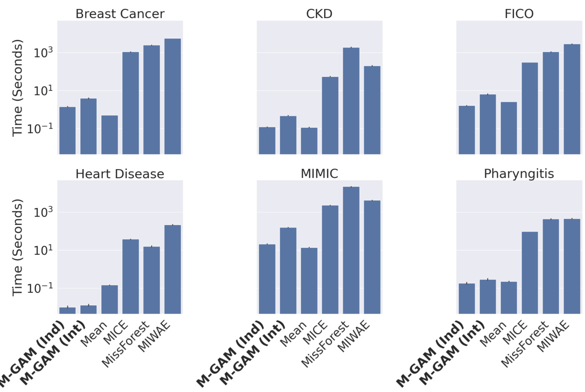
This figure compares the sparsity (number of non-zero coefficients) of M-GAM with other methods for handling missing data in GAMs, under different levels of synthetic MAR missingness (25% and 50%). M-GAM’s sparsity is significantly better than methods using multiple imputation, demonstrating its ability to achieve comparable accuracy while maintaining interpretability.
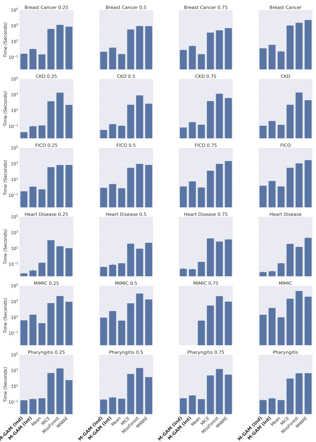
This figure compares the sparsity (number of non-zero coefficients) and accuracy (test accuracy or AUC) of M-GAM with different methods for handling missing data in the FICO and Breast Cancer datasets. Synthetic MAR missingness is introduced at rates of up to 25% and 50%. The comparison includes multiple imputation methods (MIWAE, MICE, MissForest), a GAM with 0-value imputation, a GAM with mean imputation, and a method selectively adding missingness indicators. M-GAM demonstrates its ability to achieve comparable or superior accuracy with significantly fewer coefficients compared to the other methods, showcasing its sparsity and efficiency.

This figure compares the sparsity (number of non-zero coefficients) of M-GAM with other methods for handling missing data in GAMs, under different rates of synthetic MAR missingness. It shows that M-GAM achieves similar or better accuracy with substantially fewer coefficients than alternative approaches like multiple imputation.
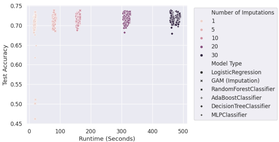
This figure compares the sparsity (number of non-zero coefficients) and accuracy (test AUC or accuracy) of M-GAM with several baseline methods for handling missing data in two datasets (FICO and Breast Cancer) under different rates of synthetic MAR missingness (25% and 50%). The baselines include multiple imputation methods (MIWAE, MICE, MissForest), GAM with 0-value imputation, GAM with mean imputation and a method that selectively adds missingness indicators. M-GAM demonstrates superior sparsity while maintaining comparable or better accuracy than the alternatives.
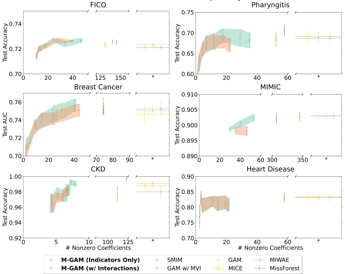
This figure compares the sparsity (number of non-zero coefficients) and accuracy of M-GAM with other methods for handling missing data in two datasets (FICO and Breast Cancer) under different rates of synthetic MAR (Missing at Random) missingness. It shows that M-GAM achieves comparable or better accuracy with significantly fewer non-zero coefficients than alternative methods such as multiple imputation (MICE, MIWAE, MissForest) and methods that simply add missingness indicators or use mean imputation. The results highlight M-GAM’s effectiveness in producing sparse and interpretable models, even with a substantial amount of missing data.
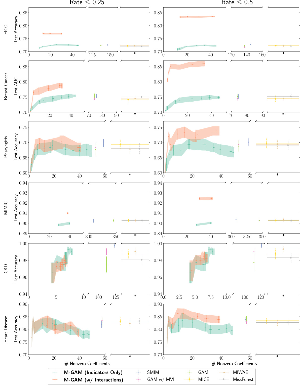
This figure compares the sparsity (number of non-zero coefficients) and accuracy (test accuracy for FICO and test AUC for Breast Cancer) of M-GAM with and without interaction terms to several other methods for handling missing data in GAMs. These methods include multiple imputation techniques (MICE, MIWAE, MissForest), a simple GAM with 0-imputation and mean-value imputation, and a model that adds only missingness indicators. The results show that M-GAM achieves similar or superior accuracy to these methods while having substantially fewer non-zero coefficients, demonstrating its effectiveness in producing sparse and accurate models, especially when handling synthetic MAR missingness. Error bars represent the standard error calculated over 10 train-test splits.
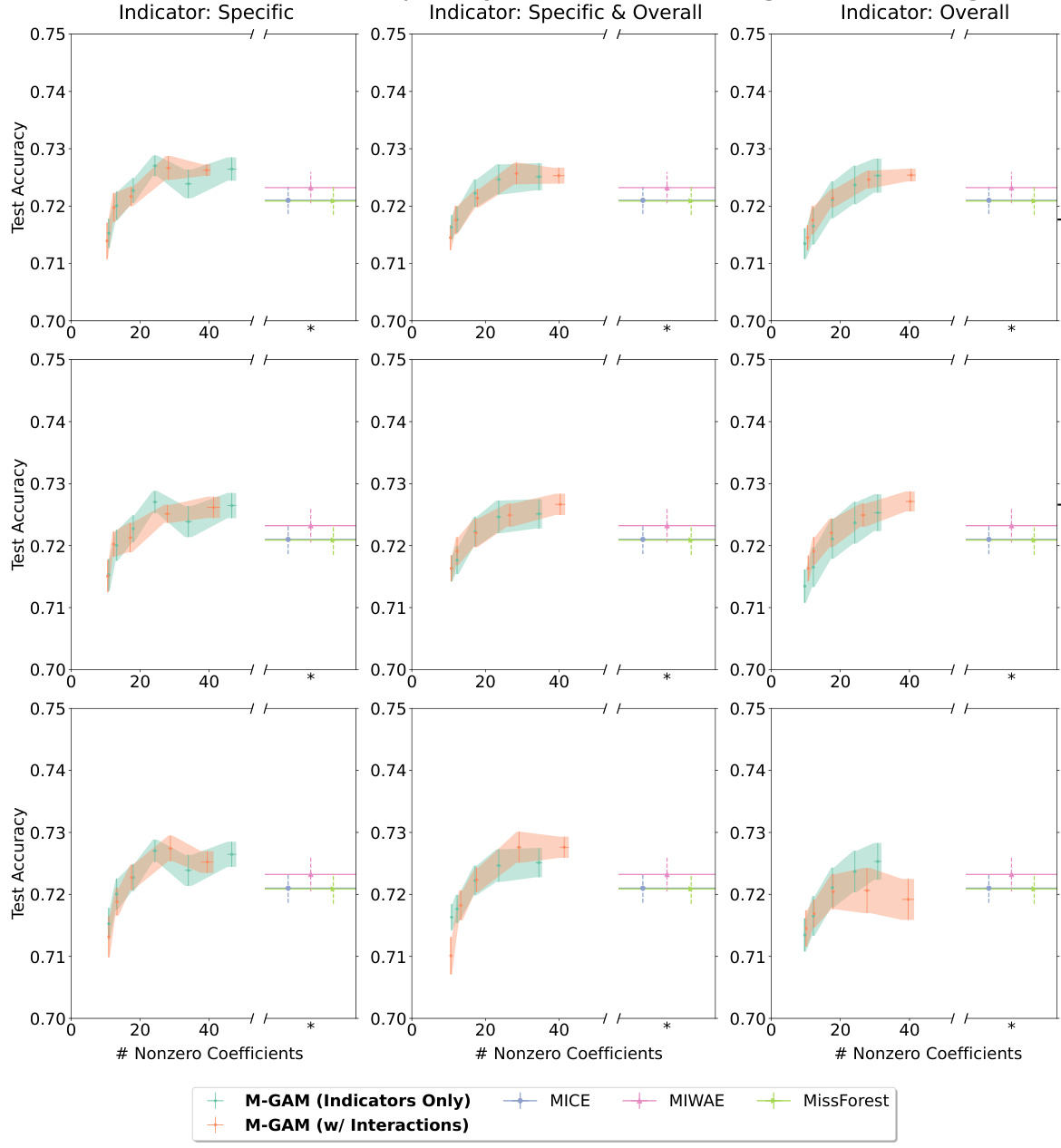
This figure compares the sparsity and accuracy of M-GAM against other methods for handling missing data in GAMs. It shows how the number of non-zero coefficients (a measure of sparsity) changes with increasing rates of synthetic MAR missingness (25% and 50%) in the FICO and Breast Cancer datasets. Multiple imputation methods (MICE, MIWAE, MissForest) and simpler methods (0-value imputation, mean-value imputation, selective addition of indicators) are also compared. M-GAM demonstrates better sparsity while maintaining comparable or superior accuracy.

This figure shows a generalized additive model (GAM) that incorporates missing data handling directly into its reasoning process. It demonstrates how the model adjusts its shape functions for a variable based on whether other variables have missing values and the type of missingness encountered. The method uses simple adjustments to existing shape curves when a value is missing, enhancing interpretability. It avoids the complexities associated with imputation or simply adding indicator variables, making it efficient for analyzing datasets with missing values.

This figure shows a generalized additive model (GAM) for the Explainable ML Challenge data from FICO et al. (2018) with missingness incorporated. The model handles missingness interpretably by explicitly providing alternative shape functions when a variable is missing. For example, the shape function for variable 2 is adjusted when variable 3 is missing, and the shape function for variable 3 is removed. This figure shows how the model handles missing values of different features and displays the shape functions for each feature both when data is present and when different features have missing values.

This figure shows a generalized additive model (GAM) for the Explainable ML Challenge data from FICO et al. (2018) with missingness incorporated. The left section illustrates shape functions for features under different missing data scenarios. The right section displays the shape functions which are not missingness-dependent. The M-GAM handles missingness interpretably by explicitly providing alternative shape functions when a variable is missing. For example, the shape function for variable 2 is adjusted when variable 3 is missing, and the shape function for variable 3 is removed. This illustrates the interpretability of M-GAM, which maintains global interpretability (the entire model can easily be inspected) and local interpretability (the shape functions applied for a given sample can be easily visualized).

This figure visualizes an M-GAM model applied to the Breast Cancer dataset. It shows how the model’s shape functions (which represent the relationship between each feature and the outcome) change based on whether data is missing for certain features. The left side displays the adjustments made to the shape functions when data for a specific feature is missing. The right side shows the standard shape functions applied when no data is missing. The figure illustrates the M-GAM’s interpretability by showing how its model adapts to handle missing values, while still being straightforward to interpret.
Full paper#
