↗ OpenReview ↗ NeurIPS Homepage ↗ Chat
TL;DR#
Many AI applications require incorporating human knowledge, often represented as probability distributions. However, eliciting these distributions directly from human experts is challenging, especially for high-dimensional data where humans are poor at assessing covariance structures and current methods are limited to simple forms. Existing techniques often fail to accurately capture the belief density due to problems like ‘collapsing’ or ‘diverging’ probability mass during the training process. This paper proposes a solution to this problem.
The proposed method uses normalizing flows—a type of neural network—to represent the belief density. It leverages preferential data, obtained by asking experts to compare or rank different options, rather than directly querying the probability density. A key innovation is the introduction of a novel functional prior for the normalizing flow, derived from decision-theoretic principles, that prevents the undesirable behavior of the probability mass. Empirical experiments show that this approach successfully infers the expert’s belief density, including for a large language model’s prior on real-world data, demonstrating the method’s ability to handle both synthetic and real-world datasets.
Key Takeaways#
Why does it matter?#
This paper is important because it tackles a critical challenge in AI: eliciting complex probability distributions from human experts or other information sources. Current methods are limited to simple distributions. This work introduces a novel approach using normalizing flows and preferential comparisons, opening new avenues for building more accurate and flexible models for AI systems that rely on human knowledge. This has broad implications for many applications, including reward modelling, Bayesian inference, and decision making.
Visual Insights#

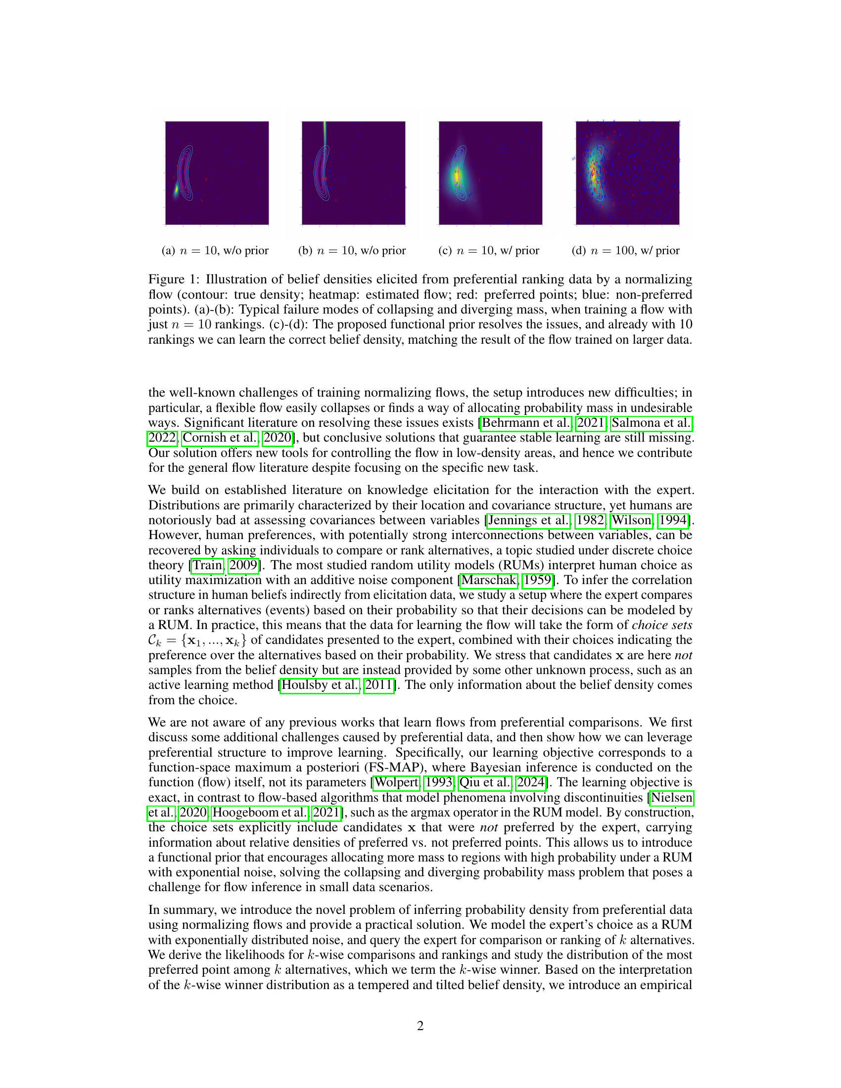
This figure shows how a normalizing flow can be used to elicit a probability distribution from an expert’s preferences. The top row shows failure cases when only 10 rankings are used. The bottom row shows that by introducing a functional prior, the method can recover the correct density even with limited data.

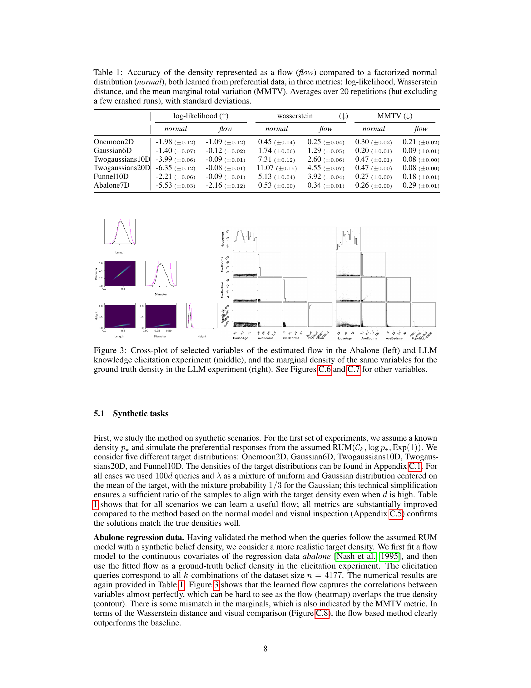
This table presents a comparison of the accuracy of representing a belief density using a normalizing flow versus a factorized normal distribution. The comparison is made across three metrics: log-likelihood, Wasserstein distance, and mean marginal total variation (MMTV). The results are averaged over 20 independent repetitions, excluding a small number of runs that experienced errors.
In-depth insights#
Pref. Data Challenges#
The challenges posed by preferential data in machine learning, particularly within the context of density estimation using normalizing flows, are multifaceted and significant. Data sparsity is a major hurdle; preferences, unlike direct samples from a distribution, are inherently limited in their information content. Each preference comparison or ranking only reveals relative probabilities, not absolute values, leading to inherent ambiguity. This ambiguity makes it difficult to accurately estimate the underlying probability density, particularly in high-dimensional spaces. Furthermore, model collapse or divergence become significant problems; flexible models like normalizing flows can easily overfit to the limited data, leading to unrealistic densities concentrating probability mass in unintended regions or failing to capture the full range of probabilities. The problem is compounded by the fact that the candidates being compared aren’t random samples from the target distribution, but rather come from an unknown, potentially non-representative, source. Therefore, a direct application of standard density estimation or variational inference techniques is not feasible. Overcoming these challenges requires innovative approaches, such as incorporating robust priors to guide model learning and prevent overfitting, and careful design of elicitation queries to maximize information gain from each preference judgment.
Flow Prior Design#
Designing effective priors for normalizing flows is crucial for successful density estimation, particularly when dealing with limited data, as in expert knowledge elicitation. A poorly chosen prior can lead to model collapse or divergence, hindering accurate belief density representation. This paper tackles this challenge by introducing a novel functional prior for the flow. This prior is decision-theoretic, rooted in a random utility model that reflects how humans make choices based on their beliefs. The prior’s design directly incorporates the structure of preferential data by focusing on the most preferred points (winners) from multiple comparisons. This approach is empirical, using the k-wise winner distribution as a basis, and elegantly addresses the problems of collapsing or diverging mass by focusing probability mass towards higher probability regions. The prior’s incorporation into a function-space maximum a posteriori (FS-MAP) estimation framework provides a principled and robust learning approach. This innovative approach significantly improves the learning process, enabling accurate density inference even from a limited number of preferential judgments.
FS-MAP Inference#
Function-space maximum a posteriori (FS-MAP) inference offers a novel approach to learning the parameters of a normalizing flow by directly optimizing the posterior distribution over the function space, rather than the parameter space. This method is particularly advantageous when dealing with limited data, such as in expert knowledge elicitation where only preferential comparisons or rankings are available. By directly modeling the posterior over the function space, FS-MAP effectively incorporates prior knowledge about the desired properties of the belief density, such as smoothness or concentration around preferred regions. This is crucial as it helps mitigate the challenges of collapsing or diverging probability mass commonly encountered when training flexible models like normalizing flows with limited data. The functional prior used in FS-MAP plays a vital role in shaping the posterior distribution, guiding the learning process towards more realistic and informative belief densities, thereby enhancing robustness. Empirical evaluations show the effectiveness of FS-MAP in accurately inferring belief densities from preferential data, even with small sample sizes.
LLM as Expert#
Utilizing a Large Language Model (LLM) as an expert source presents a compelling avenue for eliciting high-dimensional probability distributions. This approach sidesteps the limitations of relying solely on human experts, who may struggle with complex multivariate assessments or be limited by time constraints. The LLM, in this context, serves as a readily available, tireless source of probabilistic information. However, crucial considerations arise concerning the biases and limitations inherent in LLMs. The LLM’s belief density is not a ground truth; rather, it reflects the patterns and information encoded within its training data, potentially including biases present in that data. Therefore, the elicited distribution is a reflection of the LLM’s knowledge, not an objective measure of reality. This approach’s success hinges on the quality and breadth of the LLM’s training data, making careful selection of the model and rigorous validation of its outputs crucial. The process also necessitates a critical evaluation of how well the LLM’s internal representation of uncertainty maps onto true probabilistic uncertainty.
Future Extensions#
Future research could explore several promising avenues. Extending the methodology to handle more complex preference elicitation tasks such as partial rankings or pairwise comparisons with confidence levels would enhance the model’s practical applicability. Investigating different noise models beyond the exponential distribution, and exploring non-parametric approaches to model the expert’s utility function are crucial. Developing more efficient inference techniques that scale better to high-dimensional data and larger datasets is a key challenge. The current function-space MAP approach, while effective, may benefit from more sophisticated techniques. Incorporating active learning strategies would greatly improve efficiency by strategically selecting the most informative queries. Finally, evaluating the method’s performance on diverse real-world applications and comparing it against existing knowledge elicitation methods is essential to demonstrate its practical utility and robustness.
More visual insights#
More on figures
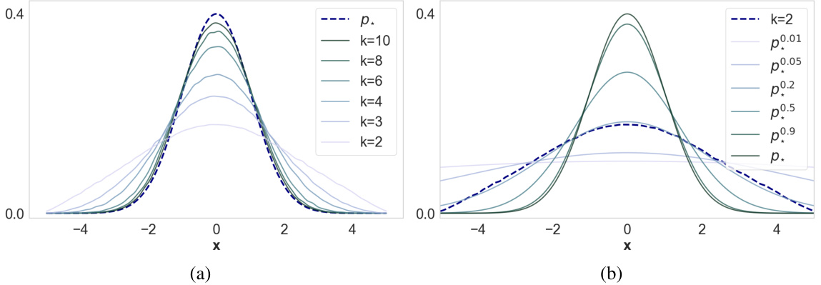
This figure shows that the k-wise winner distribution (the distribution of the most preferred point in k-wise comparisons) approaches the true belief density as k increases. Panel (a) demonstrates this convergence. Panel (b) shows that the k-wise winner distribution can also be approximated by a tempered belief density (a belief density adjusted by raising it to a power), illustrating an alternative way to represent the belief density using the k-wise winner distribution.

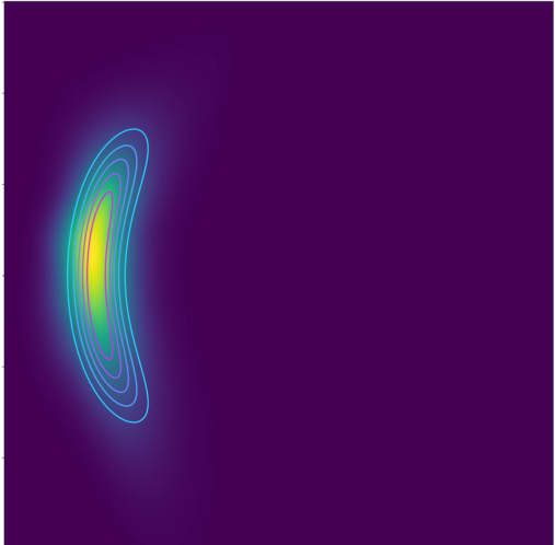
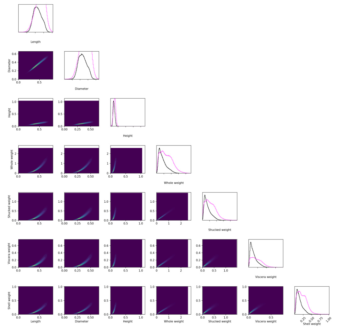
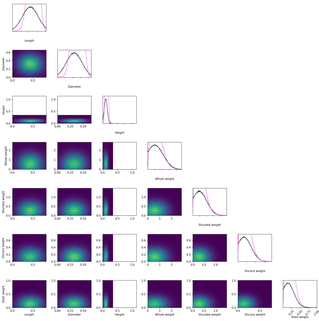
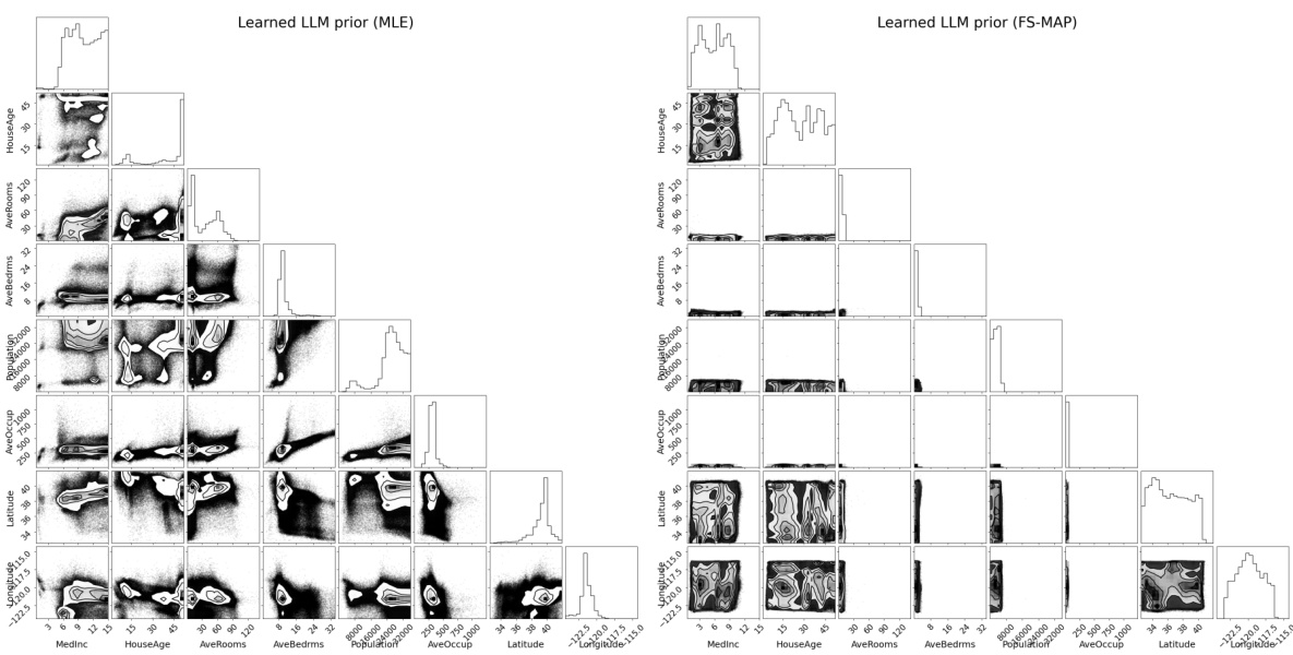
This figure shows the visualization of the learned belief density. The left panel shows the cross-plot of selected variables for the Abalone dataset. The middle panel shows the cross-plot of selected variables for the LLM experiment. The right panel shows the marginal density of the same variables for the ground truth density in the LLM experiment. Additional variables’ plots are available in Figures C.6 and C.7. This visual comparison helps to assess the quality of the learned belief density.
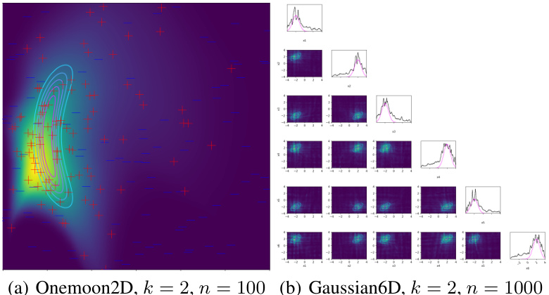
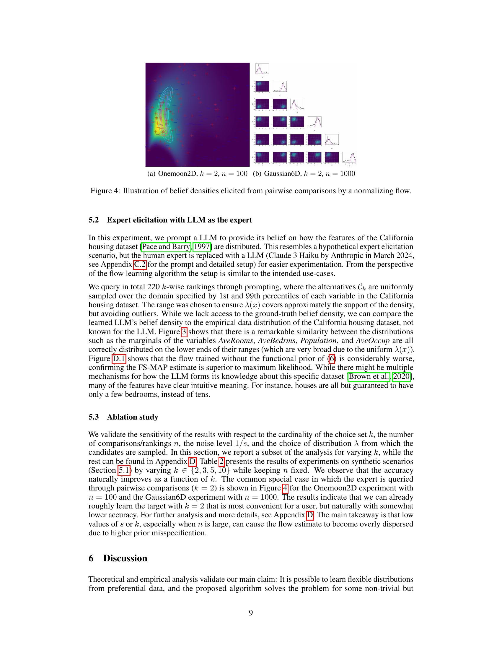
This figure shows two examples of belief densities inferred using a normalizing flow from pairwise comparisons. The left panel (a) displays the results for the Onemoon2D dataset, while the right panel (b) presents the results for the Gaussian6D dataset. Each panel shows the estimated density (heatmap) alongside a set of points representing expert preferences (red for preferred points and blue for non-preferred points), illustrating the capability of the method in estimating probability densities from limited preferential data. The contour lines represent the true underlying density, allowing a visual comparison of accuracy.
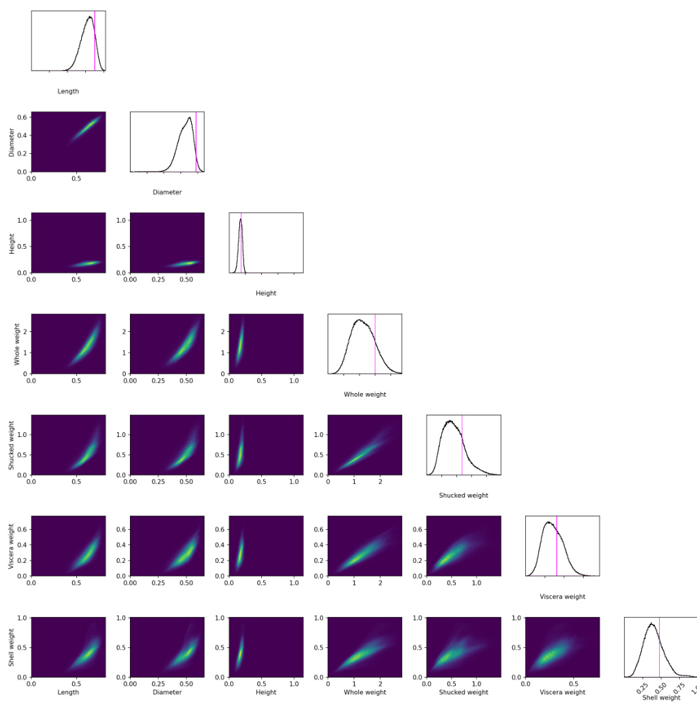
This figure shows a visual comparison of the estimated probability density (using the proposed method) with the ground truth density for selected variables. The left panel shows the Abalone dataset, the middle panel shows the LLM experiment, and the right panel shows the marginal density of the ground truth for the LLM experiment. The plots illustrate the accuracy of the learned flow in capturing the relationships between variables, and the marginal distributions compared to the ground truth.

This figure shows the results of applying the proposed method to a 6-dimensional Gaussian distribution. The contour plots show the true distribution (light blue) and the estimated distribution (dark blue). The marginal distributions are also shown (pink for true, black for estimated). The figure highlights how well the normalizing flow is able to capture the complex, high-dimensional distribution, even from limited data.
This figure shows the performance of the proposed method for eliciting high-dimensional probability distributions from an expert using preferential ranking data. Subfigures (a) and (b) illustrate common problems when training a normalizing flow with limited data: probability mass collapses to a single point or diverges widely. Subfigures (c) and (d) demonstrate that the proposed functional prior effectively mitigates these issues, leading to accurate density estimation even with only 10 rankings. The contours represent the true density, while the heatmaps show the estimated density from the normalizing flow. Red points indicate preferred alternatives, and blue points indicate non-preferred alternatives.

This figure shows the results of applying the proposed method to a synthetic 10-dimensional dataset with two Gaussian distributions. The plot visualizes both the true distribution (light blue) and the learned distribution from the preferential ranking data using normalizing flows (dark blue). Marginal distributions are also shown (pink and black curves) to provide a comparison of each individual dimension.
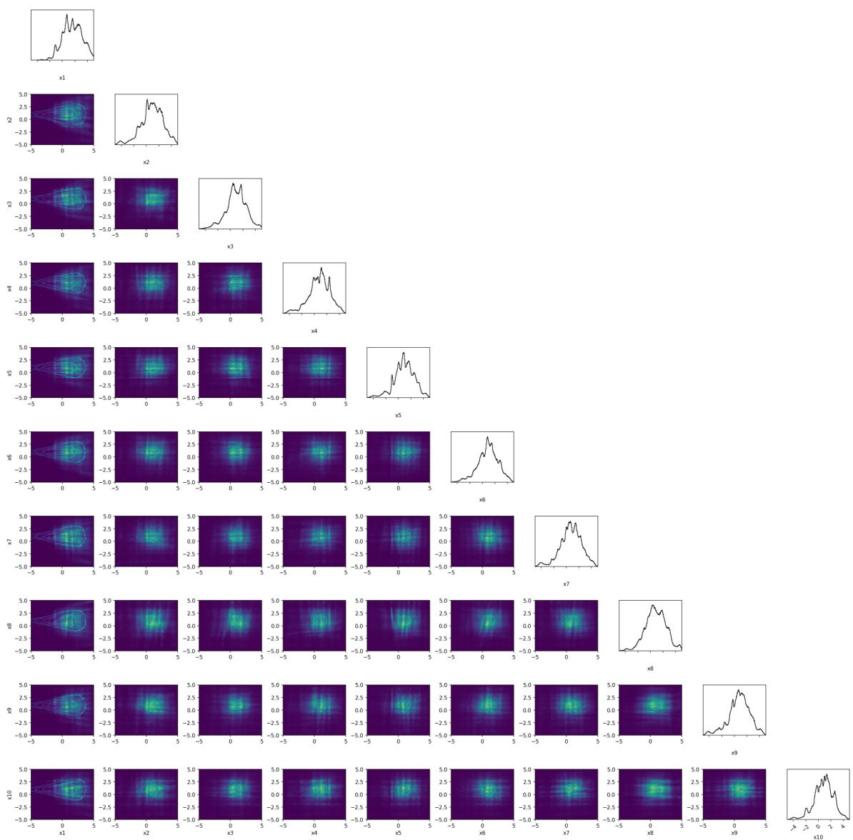
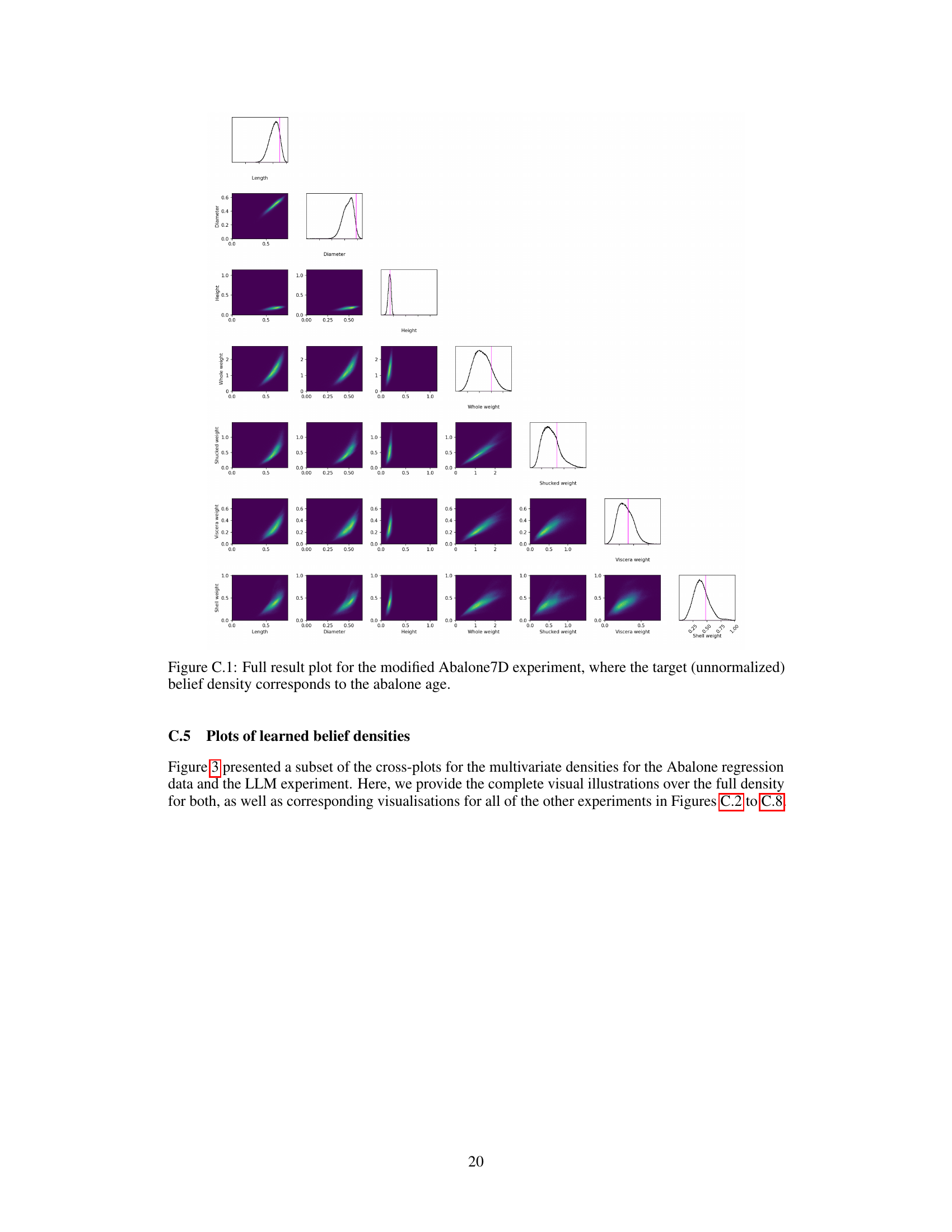
This figure shows the full result of the Abalone7D experiment, which is a more realistic synthetic dataset created by using a real-world regression dataset. It complements a smaller visualization shown earlier in the paper. The plot compares the true density (light blue) and the learned flow density (dark blue). The target and estimated densities are shown as contour lines, while marginal distributions are shown as curves. The visualization allows for a direct comparison of the learned flow to the true density.

This figure shows how a normalizing flow can be used to learn a probability distribution from preferential ranking data. The contour lines represent the true density, and the heatmaps are the densities estimated by the flow. The red points indicate preferred choices, while blue points show non-preferred choices by an expert. Panels (a) and (b) illustrate common problems when training such flows with limited data: the probability mass may collapse to a small area or spread out excessively. Panels (c) and (d) demonstrate that the proposed new functional prior for the flow effectively solves these problems, enabling accurate density estimation even with small amounts of data. This highlights the effectiveness of the authors’ method in eliciting high-dimensional belief densities.
This figure shows examples of belief densities inferred from preferential ranking data using normalizing flows. Panels (a) and (b) illustrate common problems encountered when training flows with limited data: probability mass collapses to a single point or diverges to low-probability regions. Panels (c) and (d) demonstrate that incorporating a novel functional prior addresses these issues, resulting in accurate density estimation even with only 10 rankings.
This figure shows examples of belief densities inferred from preferential ranking data using normalizing flows. Panels (a) and (b) illustrate common problems when using small datasets: probability mass collapsing to a single point or diverging to regions of low probability. Panels (c) and (d) demonstrate how the introduction of a novel functional prior solves these problems, enabling accurate density estimation even with limited data (n=10 rankings).
This figure shows the results of applying the proposed method to elicit belief densities from pairwise comparisons using a normalizing flow. It illustrates the method’s ability to capture the shape of the underlying belief density, even with a limited number of comparisons. Subfigure (a) shows the results for a two-dimensional, one-mode distribution (Onemoon2D), while subfigure (b) displays the results for a six-dimensional Gaussian distribution. The contour plots represent the true densities, the heatmaps show the learned densities, and red and blue points indicate preferred and non-preferred points, respectively. The figure showcases that the method can successfully infer high-dimensional probability distributions from preferential data.
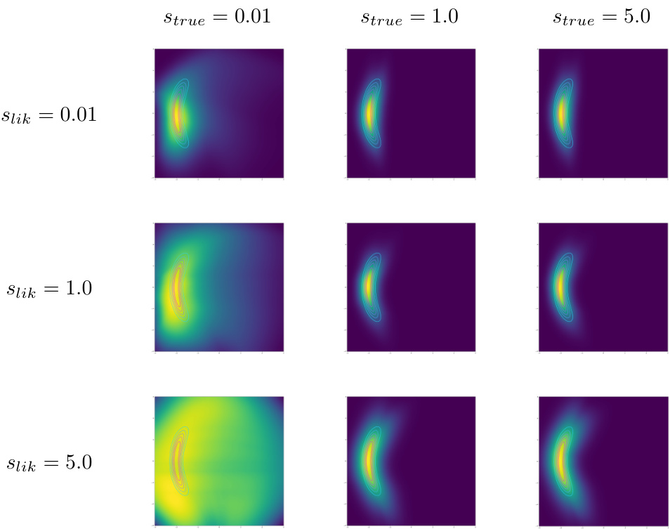
This figure shows the impact of different noise levels in the data generation process and likelihood function on the learned flow model. The results indicate that a mismatch in noise levels (between the data generating process and the likelihood) does not cause a complete failure, but rather a less accurate (more spread-out) result.

This figure shows the robustness of the proposed method to the choice of the candidate sampling distribution. The Wasserstein distance between the estimated and true densities is plotted against different mixture probabilities (w) of a uniform and Gaussian distribution used for sampling candidates. The results demonstrate that the accuracy remains high even when the sampling distribution is far from the target distribution.

This figure shows the results of the Onemoon2D experiment with different numbers of rankings (n). It displays the true density using contours and the estimated density using a heatmap for n=25, n=100, and n=1000 respectively. The figure demonstrates how increasing n improves the accuracy of the estimated density, but also shows that excessive n might lead to overestimation of the density’s spread, resulting in slightly lower accuracy.

This figure shows cross-plots of selected variables from the estimated flow in the Twogaussians10D experiment, comparing different numbers of rankings (n). The true density is represented by contour lines, and the estimated flow density is depicted as a heatmap. The marginal distributions are also shown. The results indicate that while increasing the number of rankings improves coverage, there’s also a slight increase in the spread of the estimated density, which explains a minor decrease in performance.

This figure shows the results of eliciting belief densities using pairwise comparisons with a normalizing flow. The plots showcase the learned belief densities from pairwise comparisons, illustrating the performance of the proposed method in recovering the underlying probability distributions. The figure highlights the effectiveness of the method in capturing the shape and distribution of the belief densities, even with limited pairwise comparison data.
More on tables

This table presents the Wasserstein distances for four different datasets (Onemoon2D, Gaussian6D, Funnel10D, Twogaussians10D) and four different values of k (k=2, k=3, k=5, k=10). The Wasserstein distance is a measure of the distance between two probability distributions. Lower values indicate a better fit between the estimated density and the ground truth density. The results show that the Wasserstein distance decreases as k increases, indicating that using more alternatives in the pairwise comparisons leads to a better estimation of the underlying density.

This table presents a comparison of the accuracy of representing a probability density using a normalizing flow versus a simpler factorized normal distribution. The comparison is made using three metrics: log-likelihood (higher is better), Wasserstein distance (lower is better), and mean marginal total variation (MMTV, lower is better). The results are averages over 20 independent runs, excluding a few runs that crashed due to numerical instability. The table shows results on different synthetic datasets with varying dimensionality and complexity, demonstrating the relative performance of the two methods under different conditions.

This table presents the performance comparison between the proposed normalizing flow method and a factorized normal distribution baseline in terms of three evaluation metrics. The metrics are computed for various synthetic datasets and the real-world Abalone dataset. The results highlight the superior performance of the normalizing flow method across all metrics and datasets.

The table presents the performance comparison of two methods (flow-based and factorized normal distribution) in learning probability densities from preferential data. The comparison uses three metrics: log-likelihood, Wasserstein distance, and mean marginal total variation (MMTV). Results are averaged over 20 runs (excluding those with errors), with standard deviations reported to show the variability.

This table compares the performance of the proposed normalizing flow method against a simpler factorized normal distribution baseline for estimating probability densities from preferential data. It shows the results for five synthetic datasets (Onemoon2D, Gaussian6D, Twogaussians10D, Twogaussians20D, Funnel10D) and a real-world dataset (Abalone). Three evaluation metrics are used: log-likelihood (higher is better), Wasserstein distance (lower is better), and mean marginal total variation (MMTV, lower is better). The results demonstrate that the flow model generally outperforms the simpler baseline, achieving significantly better log-likelihoods and lower distances, showcasing the advantage of more flexible models when dealing with limited data.
Full paper#

