↗ OpenReview ↗ NeurIPS Homepage ↗ Chat
TL;DR#
Non-stationary time series forecasting remains challenging due to evolving trends and seasonal patterns, limiting the effectiveness of traditional methods. Existing instance normalization techniques, while improving accuracy, struggle with complex seasonal patterns.
The proposed Frequency Adaptive Normalization (FAN) method innovatively addresses this limitation by employing Fourier transforms to identify instance-wise predominant frequencies, effectively handling both dynamic trends and seasonality. FAN then uses these identified frequencies to normalize the data, modeling the discrepancy between input and output frequencies via a simple MLP. Experiments across eight benchmark datasets show substantial improvements (7.76%~37.90% average improvements in MSE), highlighting FAN’s potential for broader applicability and improved forecasting accuracy.
Key Takeaways#
Why does it matter?#
This paper is highly important for researchers in time series forecasting due to its significant performance improvement and its novel approach of handling non-stationarity. The introduction of Frequency Adaptive Normalization (FAN) offers a model-agnostic solution applicable to various forecasting backbones, opening new avenues for researchers to enhance the accuracy of their models, especially when dealing with complex, real-world data exhibiting dynamic trends and seasonal patterns. The method’s effectiveness across multiple datasets also underscores its generalizability and practical value. Furthermore, the theoretical analysis enhances our understanding of the method’s impact on stationarity and distribution, potentially leading to further development in the area.
Visual Insights#
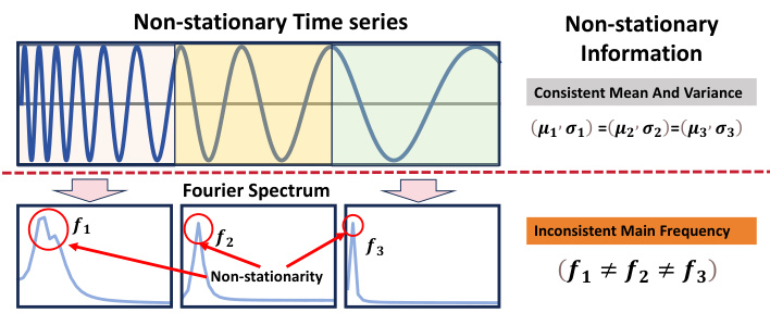
This figure shows a sinusoidal signal with a linearly varying frequency. The three segments of the signal highlight the concept of non-stationarity, because they have consistent mean and variance but different Fourier frequencies. The Fourier spectrum plots for each segment visually demonstrate the changing principal frequencies, illustrating the limitations of methods that rely solely on statistical measures (mean and variance) to capture non-stationarity.

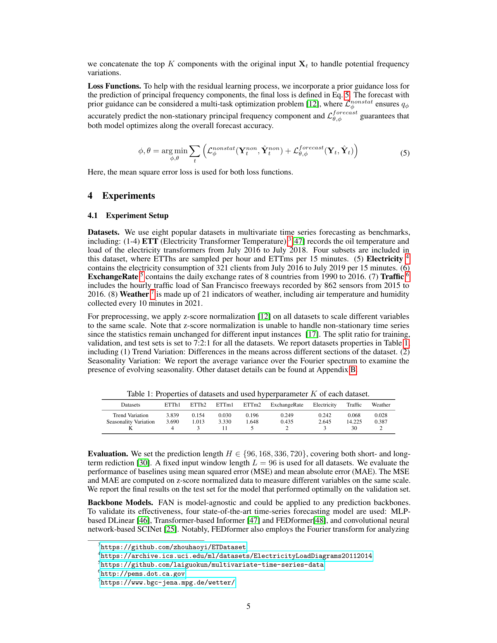
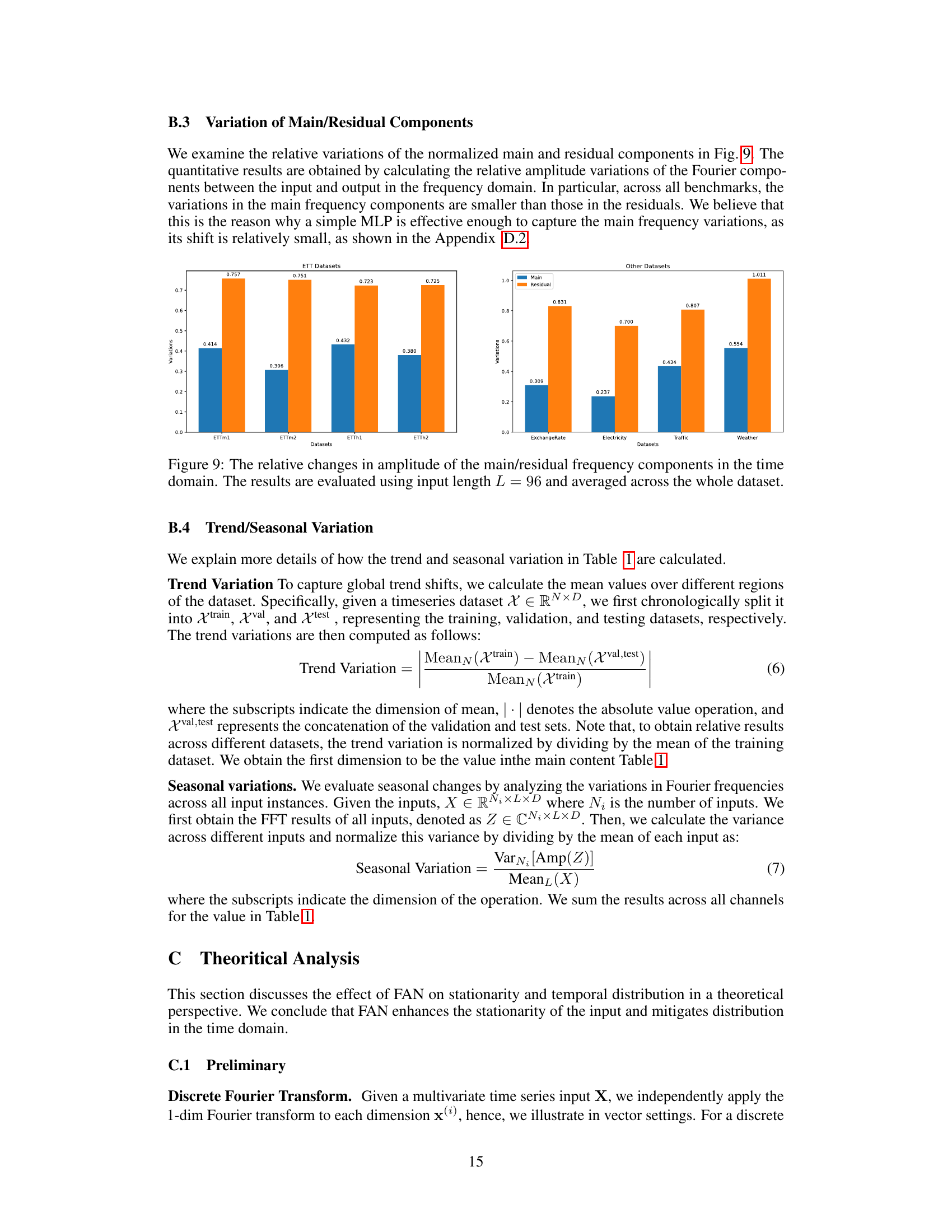
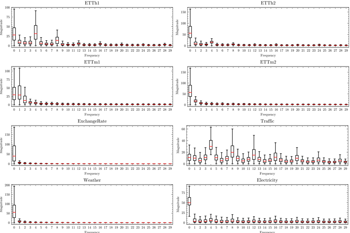
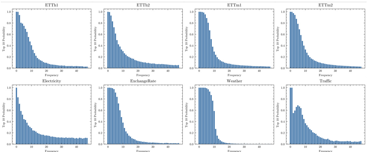
This table presents the characteristics of eight benchmark datasets used in the paper for multivariate time series forecasting. For each dataset, it shows the trend variation (differences in means across different sections), seasonality variation (average variance over the Fourier spectrum), and the chosen hyperparameter K (number of dominant frequency components considered). These values are relevant because they illustrate the varying degrees of non-stationarity present in each dataset and how the model parameters were adjusted to suit.
In-depth insights#
FAN: Core Idea#
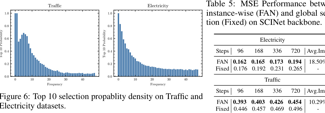
The core idea behind FAN (Frequency Adaptive Normalization) is to improve time series forecasting accuracy by addressing non-stationarity. Unlike methods relying solely on basic statistical measures like mean and variance, FAN leverages the Fourier transform to identify instance-wise predominant frequencies. This allows the model to separate stationary components from non-stationary (trend and seasonal) components, making the forecasting task easier. Crucially, FAN models the discrepancy in frequency components between input and output, unlike reversible instance normalization methods that assume consistent trends, enhancing its ability to handle dynamic patterns. By using a simple MLP to predict the changes in the prominent frequencies between input and output, FAN achieves a model-agnostic solution applicable to various forecasting backbones. This frequency-based approach allows FAN to distinguish patterns missed by simpler methods, significantly improving forecast accuracy on various benchmark datasets.
Frequency Analysis#
A thorough frequency analysis in a time series context would involve several key aspects. Firstly, identifying the dominant frequencies present in the data is crucial, often using techniques like the Fast Fourier Transform (FFT). This reveals the periodic patterns inherent in the data, such as seasonal or cyclical trends. Secondly, analyzing the amplitude and phase of these frequencies provides insights into the strength and timing of those patterns. Changes in amplitude might signify variations in the intensity of seasonal effects over time, while shifts in phase could indicate changes in the timing of those patterns. Thirdly, examining the evolution of frequencies over time is important for non-stationary time series, revealing how periodic patterns change over time. This often necessitates a time-frequency analysis, providing a visual representation of the frequency content at different time points. Finally, relating frequencies to external factors can uncover valuable connections between the periodic patterns in the data and external influences, contributing to a richer understanding of the underlying phenomena and providing a more robust forecasting framework.
Model Comparisons#
A dedicated ‘Model Comparisons’ section in a research paper would provide a crucial analysis of various models’ performance. It should go beyond simply reporting metrics; a thoughtful comparison would delve into the strengths and weaknesses of each model, considering factors like computational cost, data requirements, and the models’ inherent biases. The analysis might involve visualizations, showing how different models handle various aspects of the data, such as trends, seasonality, or outliers. Statistical significance tests would be essential to ascertain whether observed differences are truly meaningful or just random variation. Furthermore, the comparison should contextualize the models within the existing literature, highlighting how the proposed model stands out or compares against established baselines and state-of-the-art approaches. Finally, limitations of each model should be acknowledged, making the discussion comprehensive and transparent.
Ablation Studies#
An ablation study systematically removes components of a model to assess their individual contributions. In the context of a time series forecasting model, this might involve removing normalization techniques, the frequency residual learning module, or the non-stationary pattern prediction module. By progressively removing these components and observing the impact on performance metrics (like MSE or MAE), researchers can quantify the value of each component. This helps determine which parts are most crucial for the model’s effectiveness and potentially identify areas for improvement or simplification. For instance, removing the non-stationary pattern prediction module might reveal whether the model heavily relies on this component for accurate long-term predictions or whether the backbone model itself can adequately capture the non-stationarity. Similarly, removing the normalization step could highlight its role in preparing the input data for the model and in improving model stability. A well-designed ablation study should reveal the relative importance of different parts of the model, giving insights into its strengths and weaknesses. The results should also inform future model designs, allowing for the potential streamlining and optimization of the model.
Future of FAN#
The future of Frequency Adaptive Normalization (FAN) looks promising, building on its demonstrated success in handling non-stationary time series forecasting. Further research could explore more sophisticated methods for selecting the principal frequency components, moving beyond simple top-K selection to incorporate more nuanced criteria based on frequency distribution characteristics or even machine learning techniques. Improving the prediction module to better capture the dynamics of evolving non-stationary patterns could also greatly enhance the model’s accuracy. This could involve incorporating more advanced neural network architectures or exploring alternative techniques such as recurrent neural networks or transformers. Addressing limitations such as handling signals with complex, non-periodic non-stationarities and reducing the reliance on the Fourier transform is also crucial to expanding FAN’s applicability. The development of efficient GPU-accelerated algorithms is essential for the scalability and practical use of FAN on larger datasets. Finally, investigating potential applications in diverse domains beyond the benchmarks tested – such as finance, healthcare, or environmental science – would showcase the general applicability of FAN and inspire further development and refinement.
More visual insights#
More on figures
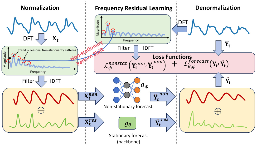
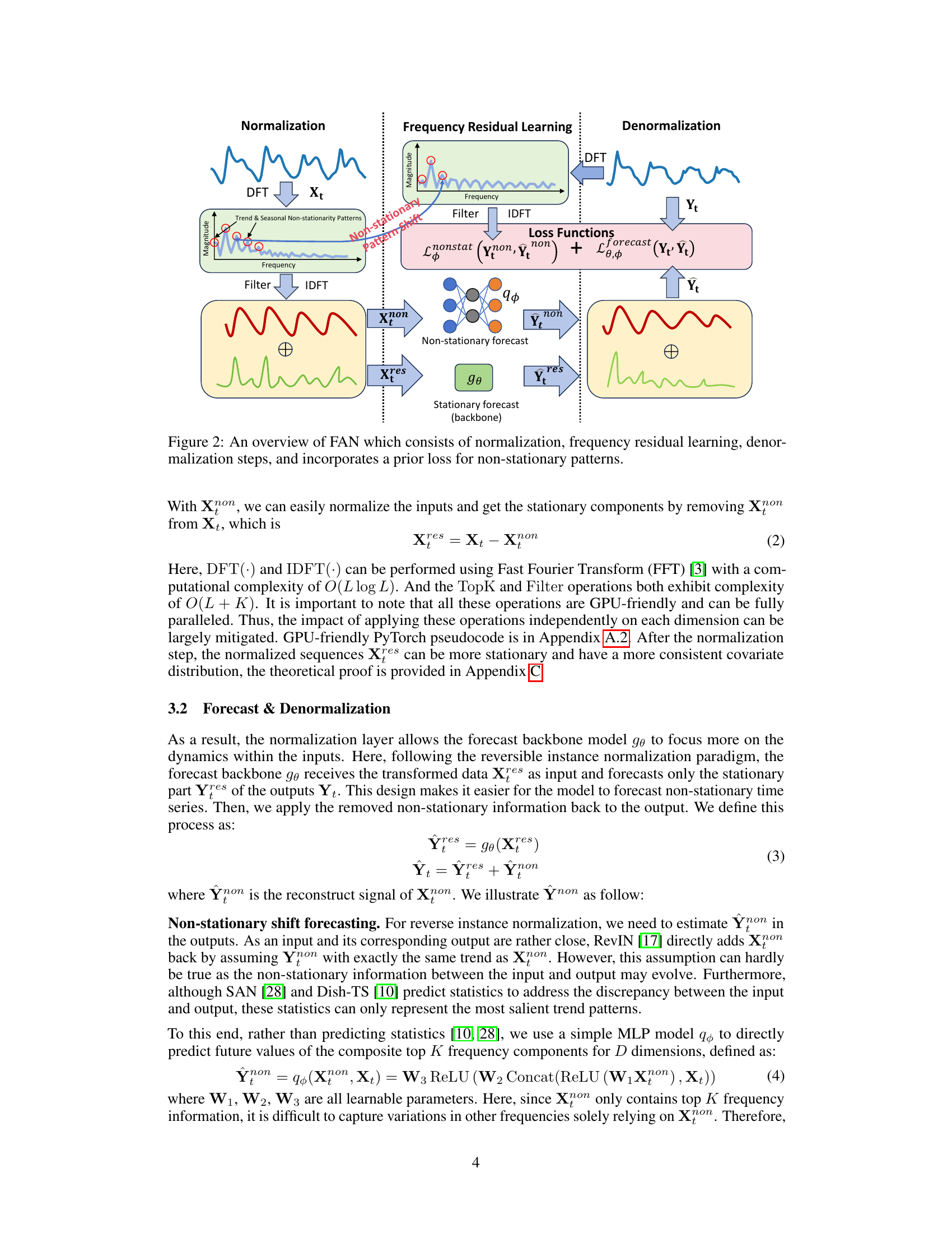
This figure illustrates the architecture of the Frequency Adaptive Normalization (FAN) method. The process begins with a normalization step, where the input time series (Xt) undergoes a Discrete Fourier Transform (DFT). The top K dominant frequency components are then identified, filtered out (using the ‘Filter’ operation), and reconstructed using an Inverse Discrete Fourier Transform (IDFT). This results in two components: Xnon (non-stationary components) and Xres (stationary components). Xres is fed into a forecasting backbone model (gθ) to predict the stationary part of the output (Ŷres). Meanwhile, a separate prediction module (qφ) using a Multi-Layer Perceptron (MLP) forecasts the non-stationary components (Ŷnon) using the removed non-stationary components (Xnon) from the input, and the current input (Xt). The overall output (Ŷt) is the sum of Ŷres and Ŷnon. A combined loss function incorporates both the prediction error (Lforecast) and the accuracy of non-stationary pattern prediction (Lφnonstat) to ensure accurate forecasting.

This figure visualizes the long-term forecasting results (168 steps) for a sample from the Traffic dataset. It compares the performance of the DLinear model enhanced with four different normalization methods: FAN, SAN, Dish-TS, and RevIN. The predictions are plotted against the ground truth values. The purpose is to illustrate how each normalization method handles the non-stationary patterns in the Traffic data, specifically showing how FAN is particularly effective at identifying and capturing seasonal patterns, unlike the other methods which seem to focus more heavily on trend.

This figure illustrates the architecture of the Frequency Adaptive Normalization (FAN) method. FAN is composed of three main stages: normalization, frequency residual learning, and denormalization. The normalization stage removes the impact of non-stationary signals (trend and seasonal patterns) from the input time series using a frequency domain decomposition. The frequency residual learning stage focuses on the stationary aspects of the input time series, enabling the forecasting backbone to learn more effectively from the stationary information. The denormalization stage uses a simple MLP to predict and add back the non-stationary information from the input, addressing potential shifts in frequency components between inputs and outputs. The whole structure also incorporates a prior loss function which guides the model to accurately predict the non-stationary components, improving overall forecasting accuracy.

This figure visualizes the long-term forecasting results (168 steps) for a sample from the Traffic dataset. It compares the performance of the DLinear model enhanced with four different normalization methods: FAN, SAN, Dish-TS, and RevIN. The goal is to illustrate how each method handles the non-stationarity of the data, particularly the seasonal patterns. The figure highlights FAN’s ability to capture evolving seasonal patterns, in contrast to the other methods that either focus on trends or make overly simplistic assumptions about the relationship between input and output non-stationary patterns.
This figure illustrates the architecture of the Frequency Adaptive Normalization (FAN) method. It shows the three main steps: normalization, frequency residual learning, and denormalization. Normalization involves using a Discrete Fourier Transform (DFT) to decompose the input time series into its frequency components. Key frequency components are then filtered out, leaving a residual signal representing the stationary aspects of the data. This residual is fed into the forecasting backbone. The denormalization process uses a prediction module (MLP) to estimate and reconstruct the non-stationary components that were previously removed, and combines this with the prediction from the forecasting backbone to produce the final forecast. A loss function is applied to the entire process, including the prediction of the non-stationary components.

This figure illustrates the architecture of the Frequency Adaptive Normalization (FAN) method. It shows the three main steps: normalization, frequency residual learning, and denormalization. Normalization removes the impact of non-stationary signals from the input time series using a frequency domain decomposition. The frequency residual learning step focuses on the stationary aspects of the input. Finally, the denormalization step reconstructs the output time series using a prediction module that addresses shifts in frequency components between the input and output. A prior loss function is used to improve the accuracy of predicting the non-stationary components.
This figure illustrates the architecture of the Frequency Adaptive Normalization (FAN) method. It shows the three main stages: normalization, frequency residual learning, and denormalization. The normalization stage uses a Fast Fourier Transform (FFT) to decompose the input time series into frequency components, filtering out the top K dominant components which represent non-stationary information. The frequency residual learning stage focuses on the remaining stationary components using a forecasting backbone model. The denormalization stage then reconstructs the output time series by incorporating a predicted non-stationary pattern (using an MLP) with the stationary forecast from the backbone model. A prior loss function is used to guide the accuracy of both the non-stationary pattern prediction and the overall forecast.
This figure shows the architecture of the Frequency Adaptive Normalization (FAN) method. It consists of three main stages: normalization, frequency residual learning, and denormalization. The normalization stage uses the Discrete Fourier Transform (DFT) to decompose the input time series into its frequency components. The frequency residual learning stage then removes the top K dominant frequency components, leaving behind only the stationary components. Finally, the denormalization stage uses an MLP to predict the non-stationary components and reconstructs the output time series. The entire process incorporates a prior loss to guide the prediction of the non-stationary components, leading to improved accuracy.

This figure illustrates the architecture of the Frequency Adaptive Normalization (FAN) method. It shows the three main components: normalization, frequency residual learning, and denormalization. The normalization step uses the Fourier Transform to separate stationary and non-stationary components. The frequency residual learning component processes the stationary components. Finally, the denormalization step combines the processed stationary components with a prediction of the evolving non-stationary patterns to reconstruct the output.

This figure visualizes the long-term forecasting results (168 steps) of a single sample from the Traffic dataset. It uses the DLinear model enhanced with four different normalization methods: FAN, SAN, Dish-TS, and RevIN. The visualization helps to compare the performance of these methods, specifically highlighting their ability to capture the evolving seasonal patterns and trend changes present in the time series data. The graphs show the predicted values and ground truth values for each normalization method, allowing for a visual comparison of their respective accuracies in capturing the non-stationary dynamics.

This figure visualizes the long-term forecasting results (168 steps) for a single sample from the Traffic dataset using the DLinear model enhanced with four different normalization methods: FAN, SAN, Dish-TS, and RevIN. Each subplot displays the ground truth and predictions. The purpose is to demonstrate how FAN better captures evolving seasonal patterns (especially noticeable around weekends) compared to the other methods that focus primarily on trends.

The figure illustrates the FAN architecture, which consists of three main steps: normalization, frequency residual learning, and denormalization. In the normalization step, the input time series is decomposed into stationary and non-stationary components using the Fourier transform. The frequency residual learning step then focuses on the stationary components to predict the stationary part of the output time series. Finally, the denormalization step combines the predicted stationary components with the predicted non-stationary components to reconstruct the final output time series. A prior loss is also incorporated to guide the model’s learning process by ensuring that the predicted non-stationary components accurately reflect the true non-stationary components.
More on tables

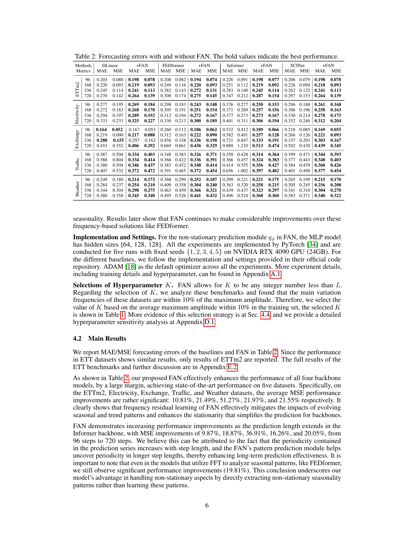
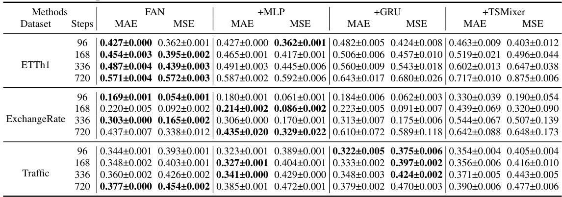
This table presents the Mean Absolute Error (MAE) and Mean Squared Error (MSE) for various time series forecasting models, both with and without the application of the proposed Frequency Adaptive Normalization (FAN) method. The results are shown for different prediction lengths (96, 168, 336, and 720 steps) across eight benchmark datasets (ETTm2, Exchange, Electricity, Traffic, and Weather). The bold values highlight the best-performing model for each metric and dataset.

This table presents a comparison of the Mean Squared Error (MSE) achieved by FAN and three other reversible instance normalization methods (SAN, Dish-TS, RevIN) across four different forecasting backbones (DLinear, FEDformer, Informer, SCINet) and eight datasets. The MSE is averaged across all prediction steps. Bold values highlight the best-performing method for each combination of backbone and dataset. This allows for an assessment of FAN’s performance improvement relative to existing normalization techniques.

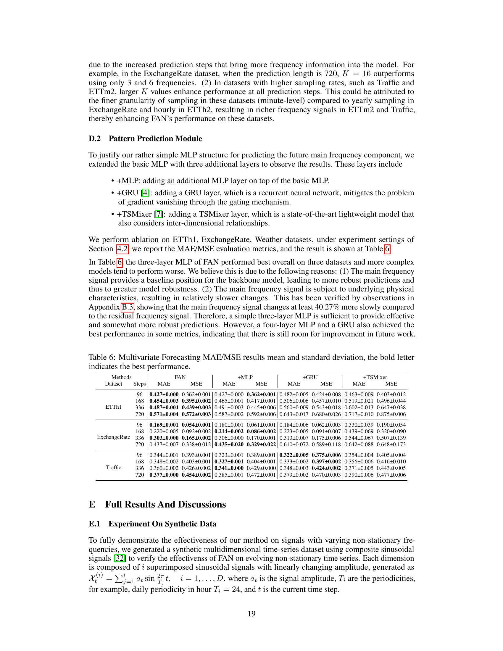
This table presents the results of ablation studies conducted on two datasets (ETTh1 and Weather) to evaluate the effectiveness of different components within the FAN model. Three variants of the FAN model are compared against the full FAN model: one without the non-stationary pattern prediction module, one using only the stationary forecasting backbone, and one without the stationary reconstruction step. The results are reported in terms of MAE and MSE for prediction lengths of 96, 168, 336, and 720 time steps, with the best performance for each metric highlighted in bold. The analysis helps to understand the relative contribution of each component of the FAN framework.
This table presents the Mean Absolute Error (MAE) and Mean Squared Error (MSE) for eight benchmark datasets across four different forecasting models (DLinear, Informer, FEDformer, and SCINet) with and without the proposed Frequency Adaptive Normalization (FAN) method. The results demonstrate the improvement in forecasting accuracy achieved by incorporating FAN with each model. The bold values highlight the best performance for each dataset and model, indicating where FAN provides the greatest benefit.

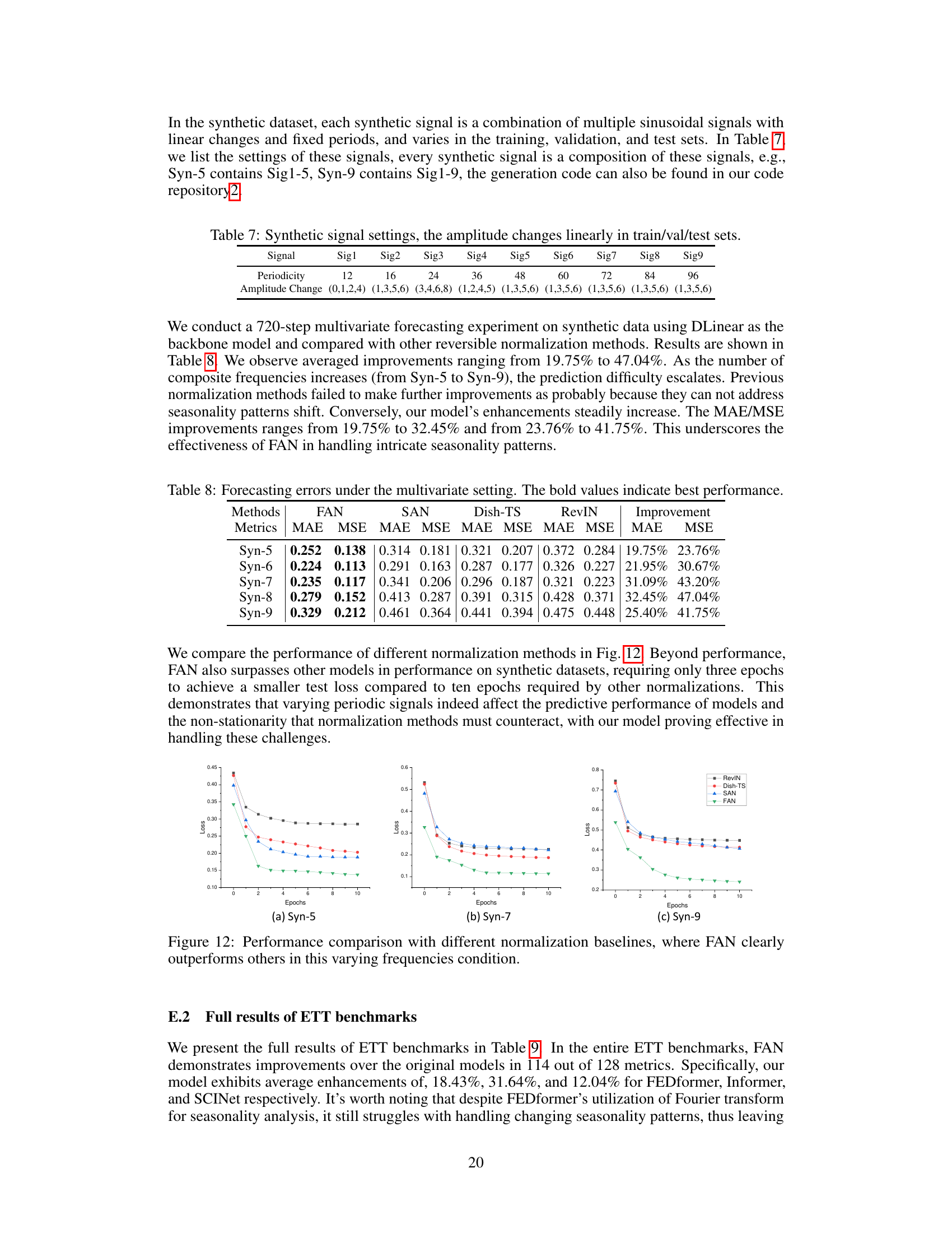
This table presents the results of a multivariate forecasting experiment on synthetic data, comparing FAN’s performance against three other reversible normalization methods (SAN, Dish-TS, RevIN). The experiment used a DLinear backbone model and varied the complexity of the synthetic time series (Syn-5 through Syn-9, reflecting an increasing number of composite frequencies). The table shows the MAE and MSE for each method and dataset, highlighting FAN’s consistent and significant performance improvements across different levels of complexity.

This table presents the results of a multivariate forecasting experiment on synthetic data using the DLinear model as the backbone. It compares the performance of FAN against three other reversible normalization methods (SAN, Dish-TS, and RevIN) across five different synthetic datasets (Syn-5 to Syn-9). Each synthetic dataset consists of a combination of multiple sinusoidal signals with linearly varying amplitudes and periodicities. The table shows the MAE and MSE for each method and dataset, highlighting the performance improvement achieved by FAN over the baselines. The improvement is expressed as a percentage increase in MAE and MSE for FAN compared to each of the other methods.
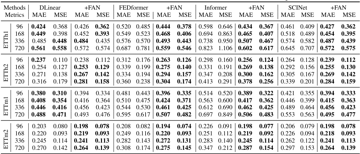
This table presents the Mean Absolute Error (MAE) and Mean Squared Error (MSE) for eight benchmark datasets, comparing forecasting models with and without the Frequency Adaptive Normalization (FAN) method. The results show the improvements achieved by incorporating FAN into various forecasting models (DLinear, Informer, FEDformer, and SCINet) across different prediction lengths (96, 168, 336, and 720 steps). Bold values highlight the best performance for each metric and prediction length.

This table presents the Mean Absolute Error (MAE) and Mean Squared Error (MSE) for eight benchmark datasets across four different forecasting models (DLinear, Informer, FEDformer, and SCINet). Each model is evaluated both with and without the proposed Frequency Adaptive Normalization (FAN) method. The results show the improvements achieved by using FAN for each model and dataset. Bold values highlight the best performance for each metric and configuration.
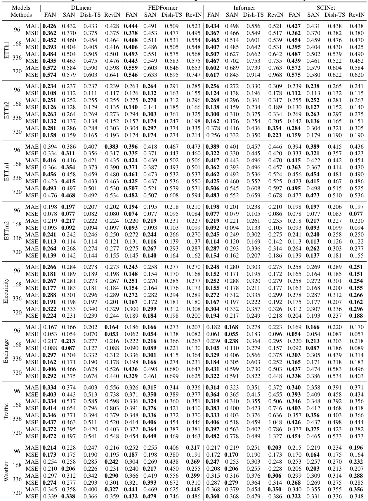
This table presents the Mean Absolute Error (MAE) and Mean Squared Error (MSE) for eight different time series forecasting datasets. The results are shown for four different forecasting models (DLinear, Informer, FEDformer, SCINet) with and without the application of the Frequency Adaptive Normalization (FAN) method proposed in the paper. The bold values highlight the best performing model for each dataset and prediction length.
Full paper#
