↗ OpenReview ↗ NeurIPS Homepage ↗ Chat
TL;DR#
Deep state space models (SSMs) are powerful for sequential data but computationally expensive due to their high state dimensions. Existing SSM architectures, including multi-SISO and MIMO structures, lack efficient dimension optimization methods. This leads to either reduced model capacity, extensive training search space, or stability issues, impacting overall efficiency and performance.
The paper proposes Layer-Adaptive STate Pruning (LAST), a structured pruning method for SSMs that minimizes model-level energy loss. LAST scores states using H∞ norms of subsystems and applies layer-wise energy normalization for cross-layer state comparison. This enables data-driven pruning decisions, optimizing SSMs across various sequence benchmarks. Results show that LAST significantly compresses SSMs (33% average state reduction) with only minor accuracy losses, demonstrating the redundancy within existing SSMs and paving the way for more efficient and stable models.
Key Takeaways#
Why does it matter?#
This paper is important because it introduces LAST, a novel structured pruning method for deep state space models (SSMs). This addresses a critical limitation of SSMs—their high computational cost due to large state dimensions—by enabling efficient model compression without retraining. This is highly relevant to current research trends in efficient deep learning and opens new avenues for improving the performance and scalability of SSMs in various applications.
Visual Insights#
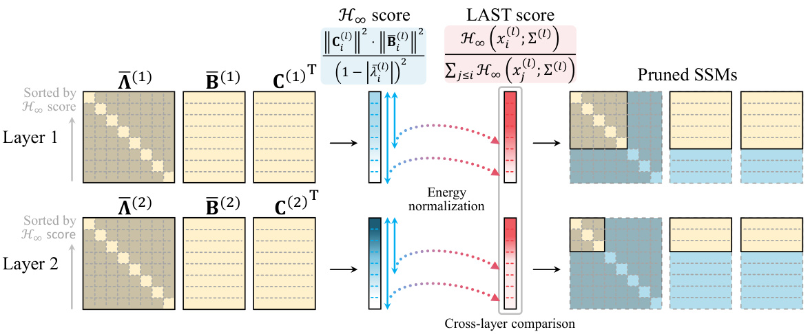
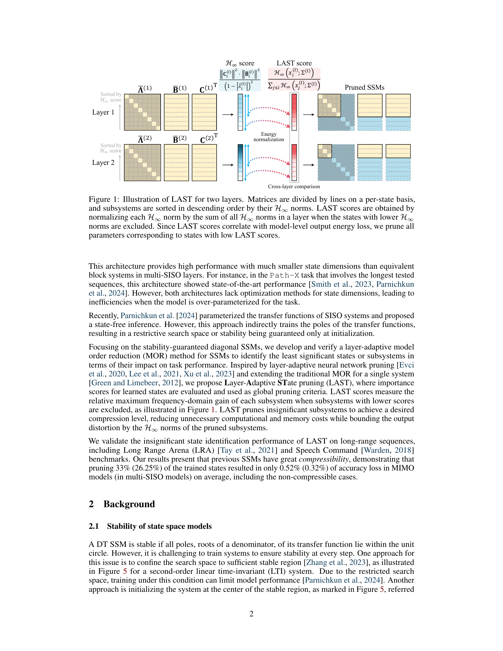
This figure illustrates the Layer-Adaptive STate pruning (LAST) method for deep state space models (SSMs). It shows how LAST works across two layers. Each layer’s matrices (A, B, C) are divided into sub-matrices representing individual states. The H∞ norm, a measure of subsystem energy, is calculated for each state. States are then sorted by their H∞ norms. LAST scores are computed by normalizing each state’s H∞ norm by the total H∞ norm within its layer. This normalization allows for cross-layer comparison of state importance. Finally, states with the lowest LAST scores (representing the least significant states) are pruned, reducing the model’s state dimensionality and computational cost.
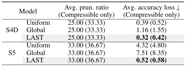
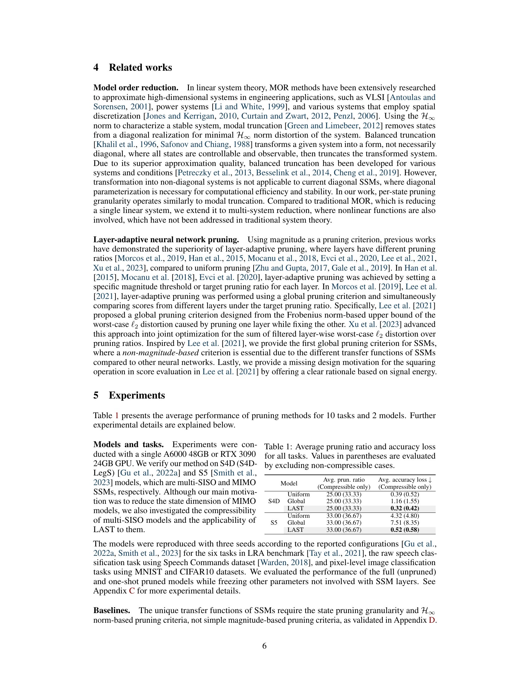
This table presents the average pruning ratio and accuracy loss for 10 tasks and 2 models (S4D and S5). The results are broken down by three pruning methods: Uniform, Global, and LAST. The numbers in parentheses show the average for only the datasets that were compressible (meaning the pruning had a reasonable effect). The table highlights that the LAST method achieves significantly lower accuracy loss compared to the other two methods at comparable pruning ratios.
In-depth insights#
Adaptive State Pruning#
Adaptive state pruning is a technique to optimize deep state space models (SSMs) by selectively removing less important states. It addresses the computational cost and memory burden associated with high-dimensional state spaces in SSMs. The adaptive nature of the pruning process is key; it dynamically determines which states to prune based on their contribution to the model’s overall performance, rather than using a uniform approach. This often involves evaluating states based on criteria such as their impact on model-level energy loss or their H∞ norms, enabling a more efficient and targeted reduction in model complexity without significantly sacrificing accuracy. The method enhances the efficiency of SSMs while preserving their expressive power. The results presented demonstrate the effectiveness of adaptive state pruning across various sequential benchmarks, achieving substantial compression without a significant loss in performance. Layer-adaptive techniques further refine this by considering layer-specific characteristics and optimizing pruning across different layers to balance compression and accuracy. The approach presents a valuable advancement for training and deploying efficient and scalable SSMs.
H∞ Norm for Pruning#
The concept of using the H∞ norm for pruning in deep state space models offers a novel approach to model compression. The H∞ norm, a measure of the worst-case gain from disturbances to outputs, provides a robust criterion for identifying less significant states or subsystems within the model. By selectively pruning these low-impact components, LAST achieves efficient model compression while bounding the output distortion, avoiding the performance degradation often associated with simpler pruning methods. This approach is particularly valuable for deep SSMs where high dimensionality can hinder training and inference. The focus on the H∞ norm leverages the tools of robust control theory, providing a theoretical grounding for the selection of states to prune. While computationally more expensive than magnitude-based pruning, the superior performance and stability guarantees suggest that the added computational cost is justified by the improved results.
MIMO SSM Efficiency#
MIMO (Multiple-Input Multiple-Output) SSMs (State Space Models) aim for efficiency by processing multiple input and output signals simultaneously, unlike multi-SISO (Single-Input Single-Output) architectures which handle each signal independently. This inherent parallelism offers potential computational advantages, particularly when dealing with high-dimensional data. However, the efficiency of MIMO SSMs is not guaranteed and depends on several factors. The choice of state dimension (n) is crucial; an overly large n can negate the benefits of MIMO processing, while an overly small n may limit model capacity and accuracy. Further, effective training techniques are essential. Poor training may cause divergence or result in suboptimal performance, offsetting any advantages of the MIMO structure. Finally, the implementation details significantly influence efficiency. For example, the specific algorithms used for matrix operations and the hardware used can significantly impact runtime. Therefore, while MIMO SSMs offer a theoretically efficient architecture, their practical efficiency requires careful consideration of state dimension optimization, robust training methodologies, and an implementation optimized for the target hardware and data characteristics.
Long-Range Sequence#
The section on “Long-Range Sequence” likely evaluates the model’s ability to handle dependencies extending across long time spans in sequential data. This is a crucial test for deep state space models (SSMs), as their performance often degrades with increasing sequence length due to vanishing or exploding gradients. The experiment likely uses datasets with long-range dependencies, such as those from natural language processing or time series forecasting, to assess how effectively the SSM captures these relationships. Positive results would demonstrate the model’s capacity to learn and maintain complex patterns over extended periods, highlighting its advantages over models struggling with long-range dependencies. Metrics such as accuracy and perplexity would probably be employed to quantify performance, with analysis focusing on whether performance is maintained or degrades at different sequence lengths. The results would be critical to validate the method’s effectiveness in real-world scenarios, where long sequences are commonplace. A comparison against alternative models known to struggle with this problem would further support the model’s strengths. Ultimately, this section aims to establish the model’s scalability and effectiveness when confronted with the inherent challenges posed by long-range dependencies in data.
Future Research#
Future research directions stemming from this Layer-Adaptive State Pruning (LAST) method for Deep State Space Models (SSMs) could explore several promising avenues. One key area is to investigate more sophisticated pruning strategies that go beyond the greedy approach, potentially incorporating techniques from reinforcement learning or Bayesian optimization for more efficient and effective state selection. Another focus could be on extending the LAST framework to different SSM architectures, such as those employing non-diagonal state matrices or recurrent neural networks. The exploration of diverse pruning granularities, beyond per-state pruning, could reveal further performance gains or efficiency improvements. Lastly, a thorough investigation into the theoretical properties of LAST, including the precise relationship between the H∞ norm and model performance after pruning, and better understanding of the stability conditions after pruning, would significantly strengthen the foundations of this work and provide valuable guidance for future SSM optimization techniques.
More visual insights#
More on figures
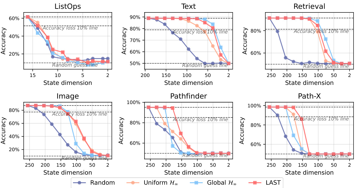
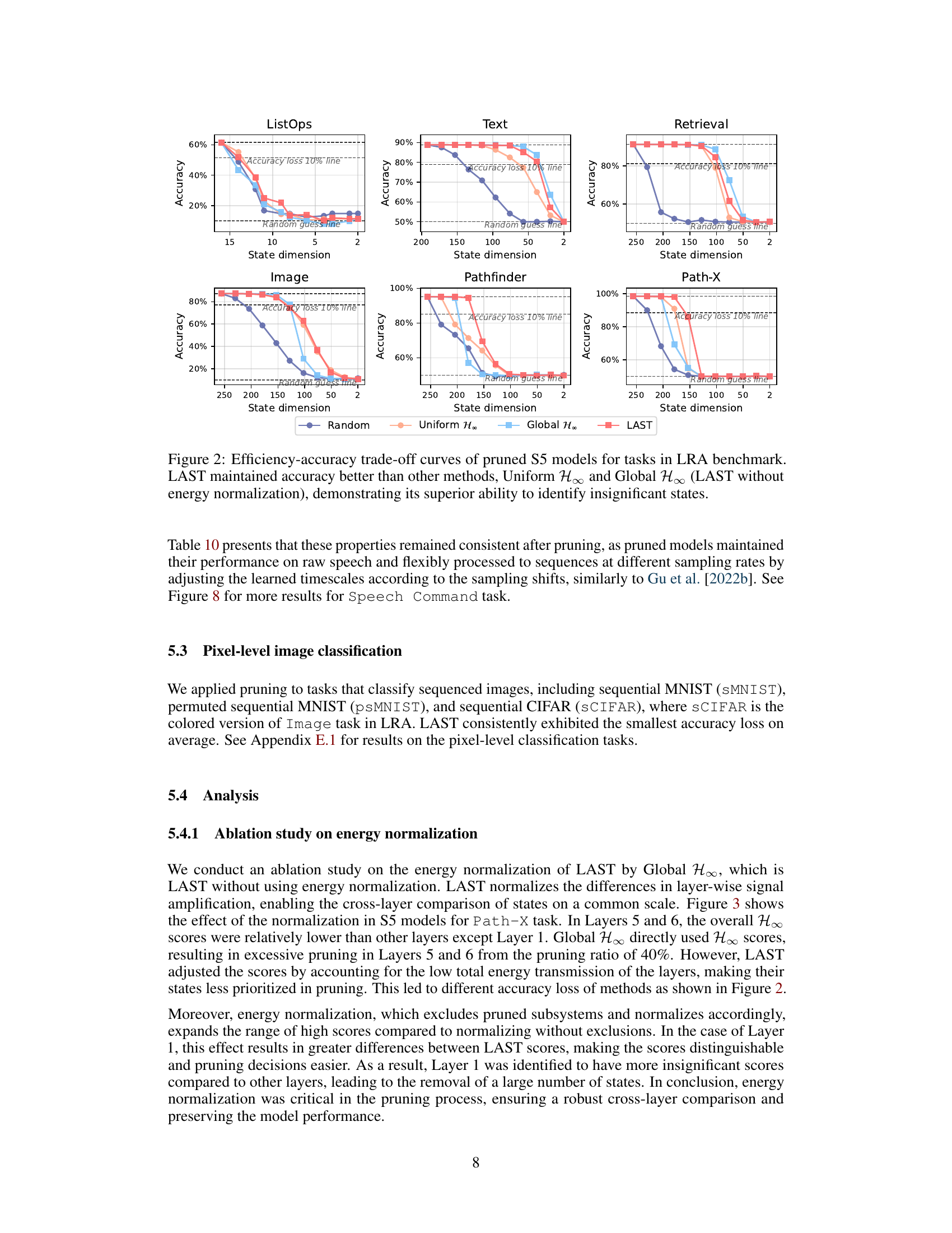
This figure displays the efficiency-accuracy trade-off curves for pruned S5 models across various tasks within the Long Range Arena (LRA) benchmark. It compares the performance of LAST against three other pruning methods: Uniform H∞, Global H∞, and random pruning. The x-axis represents the state dimension (number of states after pruning), and the y-axis represents the accuracy. The results show that LAST consistently outperforms the other methods, maintaining higher accuracy even with significant state dimension reduction. The comparison highlights the effectiveness of LAST’s layer-adaptive state pruning and the benefit of its energy normalization technique in identifying and removing less important states.

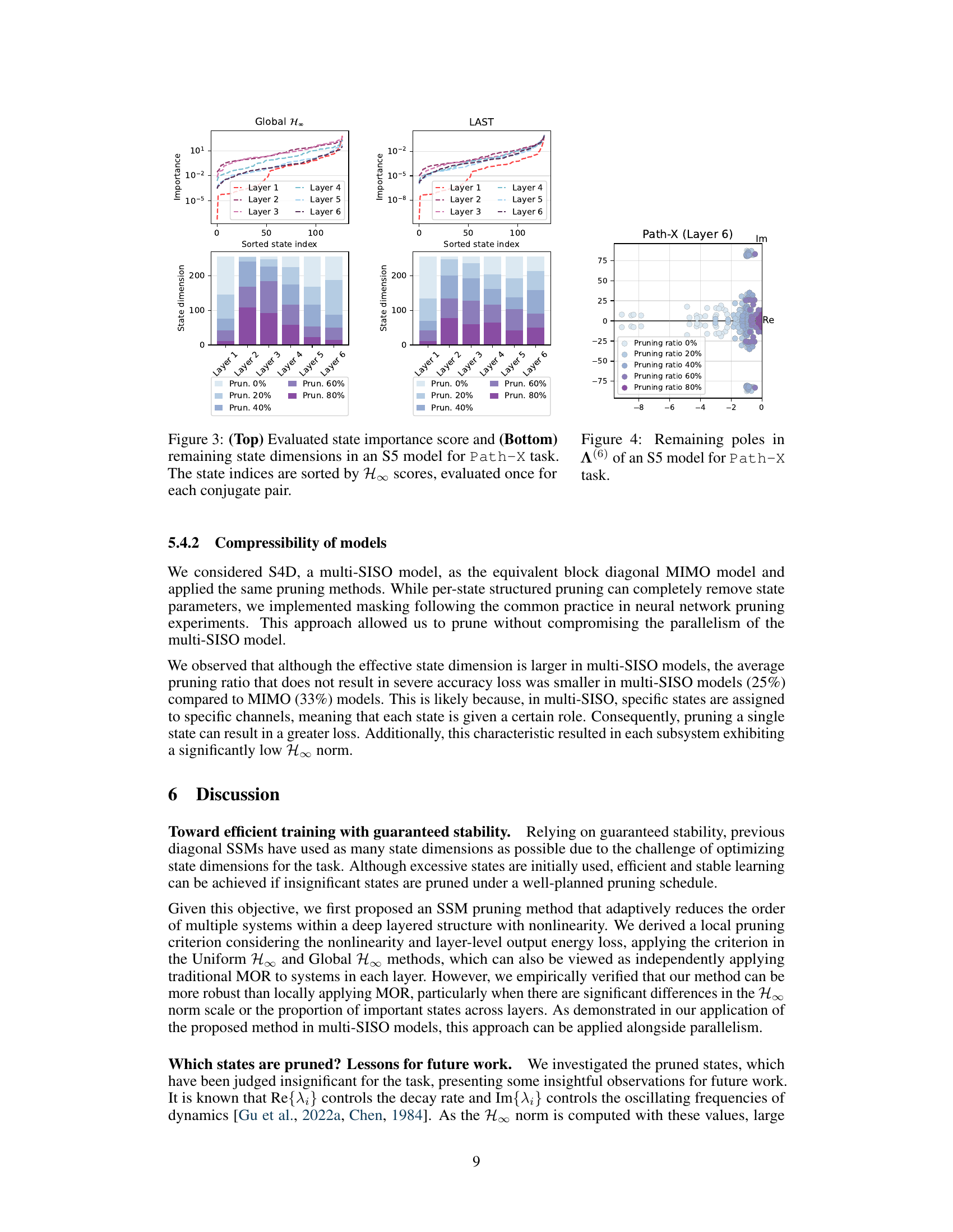
This figure shows a comparison between Global H∞ and LAST methods in terms of state importance scores and remaining state dimensions for an S5 model trained on the Path-X task. The top row displays the importance scores for each state across the six layers of the model, illustrating how LAST assigns higher scores to significant states compared to Global H∞. The bottom row presents the state dimensions remaining after pruning at different rates (0%, 20%, 40%, 60%, and 80%), showing that LAST effectively reduces the state dimension while preserving model performance. The rightmost plot visualizes the poles (complex numbers representing the system’s dynamics) for Layer 6 at different pruning ratios, further illustrating LAST’s ability to prune less significant states without affecting the model’s stability.

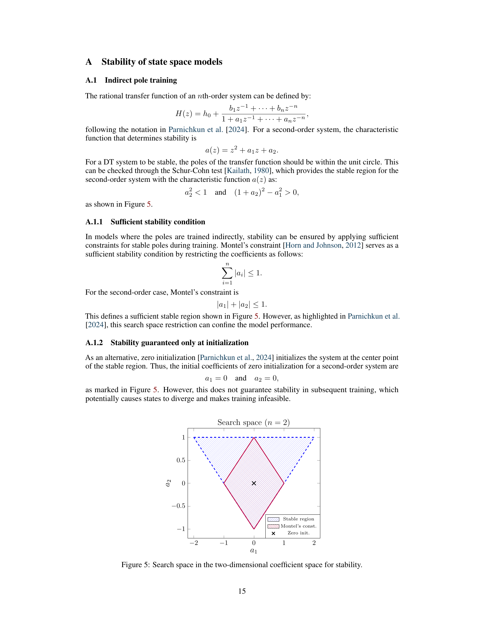
This figure illustrates the stability region for a second-order system in the two-dimensional coefficient space (a1, a2). The larger blue-shaded triangle represents the entire stability region determined by the Schur-Cohn criterion (a2 < 1 and (1 + a2)² - a1² > 0). The smaller, dark-red diamond shape within this triangle shows the stability region constrained by Montel’s criterion (|a1| + |a2| ≤ 1). The black ‘x’ marks the zero initialization point (a1 = 0, a2 = 0), highlighting that this initialization is within both stability regions. The difference in size between the regions shows the more restrictive search space imposed by Montel’s constraint in comparison to the broader Schur-Cohn criterion.

This figure compares the efficiency and accuracy of different pruning methods (random, uniform H∞, global H∞, and LAST) applied to S4D and S5 models on pixel-level image classification tasks (sMNIST, psMNIST, and sCIFAR). The x-axis represents the remaining state dimension after pruning, and the y-axis represents the accuracy. The plot shows that LAST consistently outperforms other methods in maintaining accuracy while reducing the state dimension.
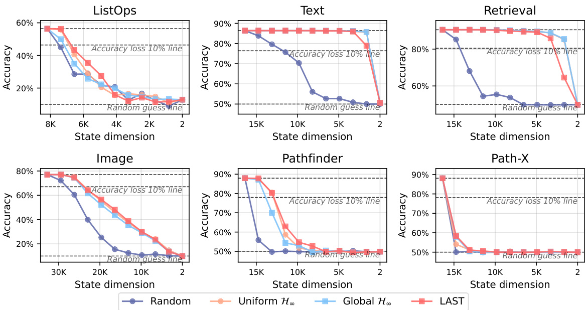
This figure shows the performance of different pruning methods (Random, Uniform H∞, Global H∞, and LAST) on various tasks from the Long Range Arena (LRA) benchmark. The x-axis represents the remaining state dimension after pruning, while the y-axis represents the accuracy. The plot demonstrates that LAST consistently outperforms the other methods in maintaining accuracy even with significant state dimension reduction, highlighting its effectiveness in identifying and removing less important states.

This figure shows the efficiency-accuracy trade-off curves for pruned S5 models across various tasks in the Long Range Arena (LRA) benchmark. The x-axis represents the remaining state dimension after pruning, and the y-axis represents the accuracy. The plot compares four methods: Random pruning, Uniform H∞ pruning, Global H∞ pruning, and LAST (Layer-Adaptive State pruning). The results demonstrate that LAST consistently outperforms the other methods, maintaining high accuracy even with significant state dimension reduction. The figure highlights LAST’s effectiveness in identifying and removing less important states, preserving model performance while reducing model complexity.
More on tables

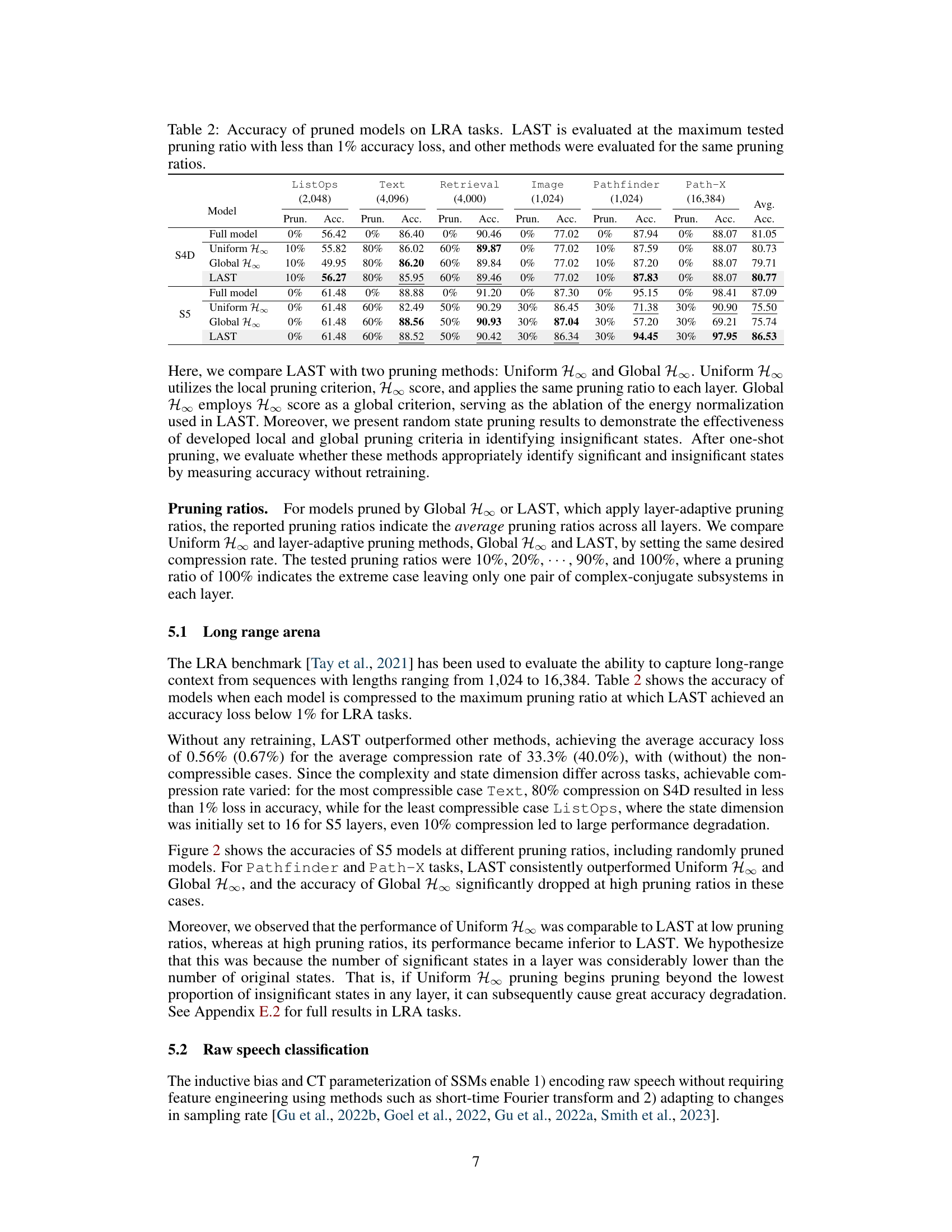
This table compares the performance of three different pruning methods (Uniform H∞, Global H∞, and LAST) on six long-range sequence tasks from the LRA benchmark. The table shows the accuracy of pruned models at different pruning ratios. The results demonstrate that LAST outperforms the other methods, maintaining high accuracy even with significant state pruning. The results highlight the effectiveness of LAST’s layer-adaptive pruning strategy and energy normalization in identifying and removing less important states.

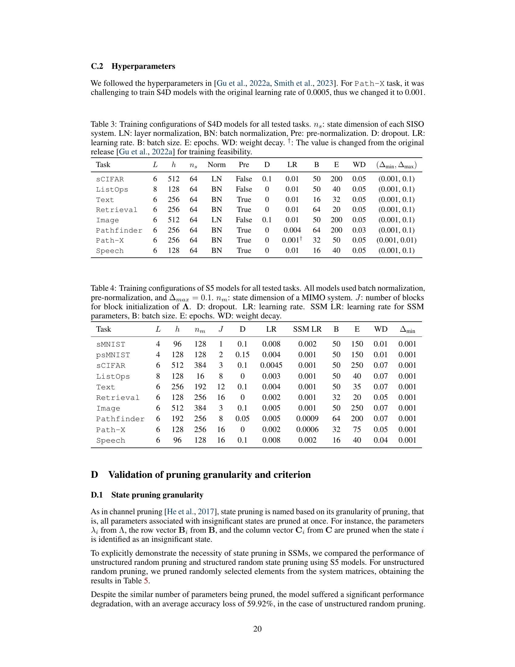
This table details the hyperparameters used for training the S4D (multi-SISO) models across various tasks. It shows the number of layers (L), input channels (h), state dimension of each SISO system (ns), normalization type (LN or BN), whether pre-normalization was used, dropout rate (D), learning rate (LR), batch size (B), number of epochs (E), weight decay (WD), and the range of timescales used (Amin, Amax). Note that the learning rate for the Path-X task was adjusted from the original setting for improved training.
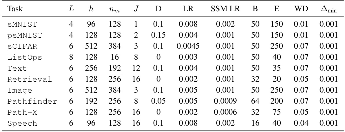
This table presents the training configurations used for the S5 models across all ten tasks in the experiments. It details hyperparameters like the number of layers (L), input channels (h), state dimension (nm), number of blocks for initialization (J), dropout rate (D), learning rates (LR and SSM LR), batch size (B), number of epochs (E), weight decay (WD), and the minimum value of A (Amin). These hyperparameters were carefully tuned to achieve optimal performance for each task.

This table presents the average pruning ratio and accuracy loss for different pruning methods across various tasks. The results are divided into two categories: all tasks and only compressible tasks. The table highlights the performance of unstructured random pruning and structured random pruning, showcasing the impact of structured pruning on maintaining accuracy.

This table compares different pruning methods (random, uniform magnitude, global magnitude, LAMP, uniform H∞, global H∞, and LAST) on S5 models across various tasks. For each method, it shows the average pruning ratio achieved and the resulting average accuracy loss. The ‘State Importance’ column shows the criteria used for pruning by each method. The values in parentheses represent results when non-compressible cases are excluded.
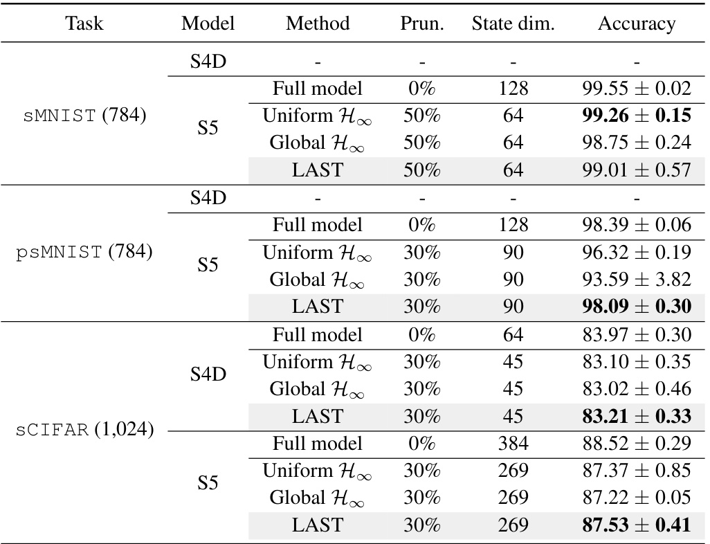
This table compares the accuracy of different pruning methods (Uniform H∞, Global H∞, and LAST) on three pixel-level image classification tasks (sMNIST, psMNIST, and sCIFAR). The results are shown for both S4D (multi-SISO) and S5 (MIMO) models. For each model and task, the accuracy is reported for the full model (no pruning) and for a pruned model at a specific pruning ratio that achieves less than 1% accuracy loss for LAST. The table highlights the superior performance of the LAST method in maintaining high accuracy after pruning compared to the other methods.

This table presents the average inference speed and peak GPU memory usage of pruned S5 models on six different tasks from the LRA benchmark. The results demonstrate the efficiency gains achieved through state pruning, showing improvements in both speed and reduced memory consumption. The degree of improvement varies depending on the specific task and the level of pruning applied.

This table compares the performance of LAST against three other pruning methods (Uniform H∞, Global H∞, and Random) across six tasks from the Long Range Arena (LRA) benchmark. The table shows the accuracy of models after applying different pruning ratios. LAST consistently demonstrates superior performance, maintaining high accuracy even with significant state pruning (up to 80% in some cases). Uniform and Global H∞ methods serve as ablations of LAST, highlighting the importance of energy normalization in LAST’s effectiveness. The Random pruning method provides a baseline showing the effectiveness of the proposed pruning strategy over a completely random approach.

This table presents the accuracy of different pruning methods (Uniform H∞, Global H∞, and LAST) on the Speech Command task, comparing their performance at various pruning ratios. The table highlights the effectiveness of LAST in maintaining high accuracy even with significant state pruning. Results are shown for both 16kHz and 8kHz sampling rates.
Full paper#
