↗ OpenReview ↗ NeurIPS Homepage ↗ Chat
TL;DR#
Deep neural networks are computationally expensive, and a key factor is layer width, which is usually determined empirically. This paper tackles this challenge by investigating how the variance of weight norm across channels changes during training. It hypothesizes that this variance pattern can indicate if a layer is wide enough.
The paper empirically shows that wide layers exhibit an “increase to saturate” (IS) pattern, where the variance increases steadily and stays high, while narrow layers show a “decrease to saturate” (DS) pattern. Based on these findings, the authors propose a method to adjust layer widths for better efficiency and performance, demonstrating that conventional wisdom on CNN layer width settings may be suboptimal.
Key Takeaways#
Why does it matter?#
This paper is crucial because it offers a novel approach to optimize the width of layers in neural networks, a long-standing challenge. It introduces a practical indicator for sufficient width, leading to more efficient models and potentially boosting performance. This is relevant to current research trends in efficient deep learning and opens avenues for further research on dynamic architecture optimization and efficient resource allocation in deep learning.
Visual Insights#

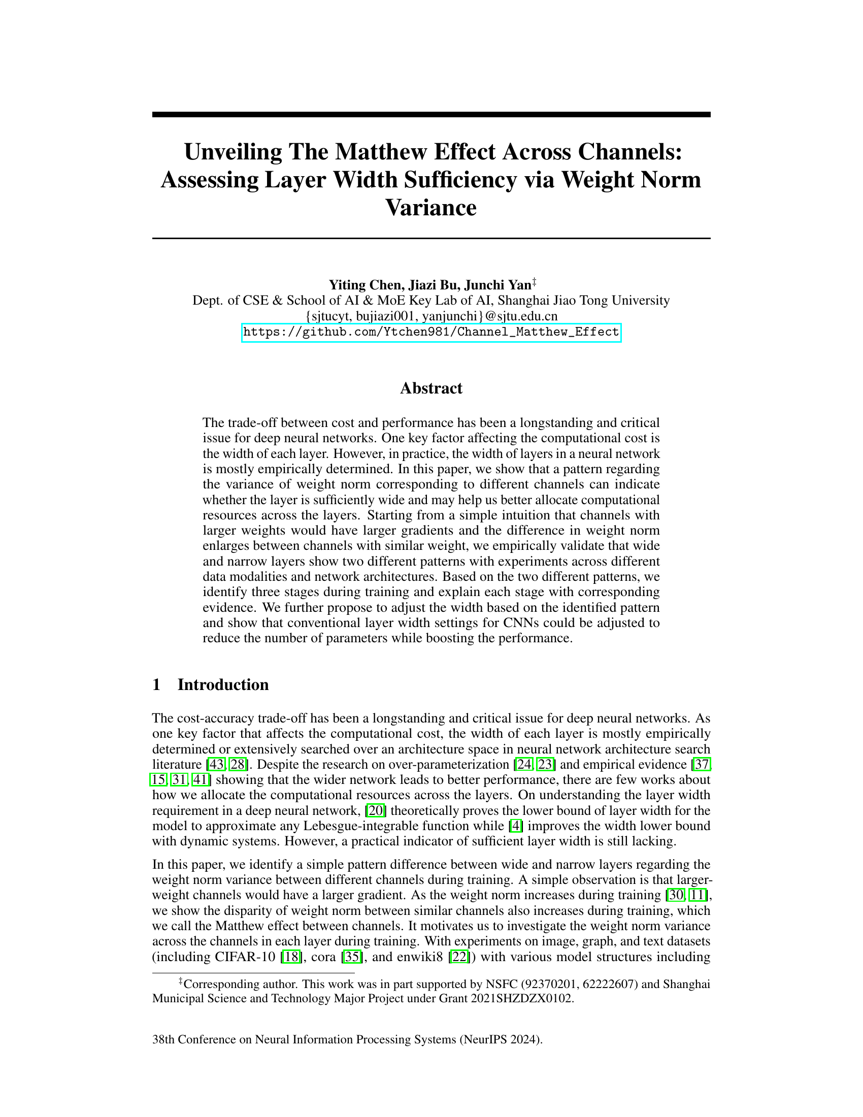
This figure illustrates the Matthew effect between channels, showing how weight norm variance changes during training for wide and narrow layers. (a) demonstrates the relationship between weight norm, gradients, and the increasing disparity between channels over time. (b) shows two distinct patterns: the increase-to-saturate (IS) pattern for wide layers and the decrease-to-saturate (DS) pattern for narrow layers, forming the basis for determining layer width sufficiency.
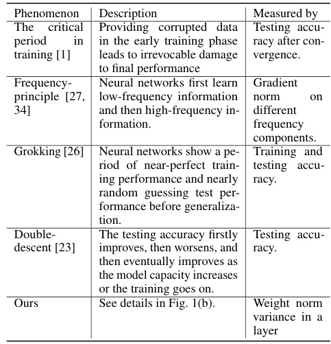
This table summarizes various phenomena observed during the training of neural networks, including the critical period, the frequency principle, grokking, double descent, and the authors’ findings on weight norm variance. Each phenomenon is described, and the metric used to measure it is specified. This helps to contextualize the authors’ work within the existing literature on neural network training dynamics.
In-depth insights#
Channel Matthew Effect#
The paper introduces the concept of “Channel Matthew Effect” to describe a phenomenon observed during the training of deep neural networks. It posits that the variance of weight norms across different channels within a layer reveals crucial information about the layer’s width sufficiency. Wide layers exhibit an “increase-to-saturate” (IS) pattern, where the variance continuously increases, suggesting adequate capacity. In contrast, narrow layers show a “decrease-to-saturate” (DS) pattern, where variance initially rises but then declines, indicating insufficient width. This effect is validated through experiments across various datasets and network architectures, highlighting a correlation between weight norm variance patterns and network performance. The authors propose adjusting layer widths based on these observed patterns to potentially optimize model efficiency, reducing parameters while enhancing performance. This insightful finding provides a practical means of assessing layer width sufficiency, going beyond existing empirical methods and offering a novel perspective for resource allocation in deep learning models.
Width-wise Streamlining#
Width-wise streamlining, as described in the research paper, presents a novel approach to optimize deep neural network architectures. The core idea revolves around adjusting layer widths based on the observed patterns of weight norm variance across channels during training. The paper identifies two distinct patterns: the increase-to-saturate (IS) pattern and the decrease-to-saturate (DS) pattern. Layers exhibiting the DS pattern are identified as candidates for width increase, suggesting that they could benefit from more parameters. Conversely, layers following the IS pattern may be sufficiently wide and thus candidates for width reduction, indicating potential for parameter efficiency gains. This dynamic width adjustment strategy, therefore, aims to strike a balance between model capacity and computational cost. The research demonstrates that this streamlining technique improves network performance while reducing the number of parameters, offering a practical and data-driven method for optimizing layer widths beyond traditional empirical or search-based approaches.
Three Training Stages#
The paper’s analysis of neural network training reveals three distinct stages: an initial phase where weight norm variance remains low due to near-orthogonal gradients, a rapid growth phase characterized by a drastic increase in both performance and variance as certain neurons’ weights dominate, and a final saturation stage exhibiting either sustained high variance (for wide layers) or a decline towards lower variance (for narrow layers). The Matthew effect, where channels with larger weights exhibit larger gradients, further explains the variance increase. The identification of these stages offers valuable insights into network training dynamics and suggests that optimal layer widths might vary depending on the training stage and desired behavior, warranting further exploration of dynamic width adjustments during training.
Norm Variance Patterns#
The analysis of weight norm variance across channels reveals two distinct patterns during neural network training: the increase-to-saturate (IS) pattern, where variance continuously increases, and the decrease-to-saturate (DS) pattern, characterized by an initial rise followed by a decline. Layer width is a crucial factor influencing these patterns; wide layers tend to exhibit IS behavior, while narrow layers display DS behavior. This observation suggests that the variance pattern serves as a valuable indicator of layer width sufficiency. Narrow layers exhibiting DS behavior could benefit from increased width, potentially enhancing performance and parameter efficiency. Conversely, layers showing IS behavior may already be sufficiently wide. This insight offers a data-driven approach to optimize layer widths during network design, going beyond traditional empirical methods, and leading to more efficient architectures.
Layer Width Dynamics#
Analyzing layer width dynamics in deep neural networks reveals crucial insights into training efficiency and model performance. Early training stages often show a gradual increase in weight norm variance, reflecting the network’s exploration of the feature space. As training progresses, wide layers tend to exhibit a sustained increase in variance, indicating sufficient capacity, while narrow layers may show a decrease after an initial rise, suggesting insufficient width and potential for improved performance with increased capacity. This observation motivates the exploration of adaptive width strategies, which dynamically adjust layer widths during training based on the observed variance patterns. This approach could lead to more efficient models with fewer parameters while maintaining or even improving accuracy by focusing computational resources where they are needed most.
More visual insights#
More on figures

This figure shows the weight norm variance changes during the training process of GCN and GRU models with varying layer widths. It demonstrates two distinct patterns: the ‘increase to saturate’ (IS) pattern for wide layers and the ‘decrease to saturate’ (DS) pattern for narrow layers. The IS pattern indicates that the weight norm variance consistently increases and remains high, suggesting sufficient layer width. Conversely, the DS pattern shows an initial increase followed by a decrease in variance, implying that the layer could benefit from increased width.
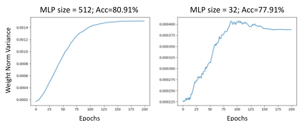
This figure shows the weight norm variance change during training for two different MLP sizes (32 and 512) within the 5th layer of a Tiny Vision Transformer (ViT) model trained on the CIFAR-10 dataset. The left panel (MLP size=512) exhibits an ‘increase to saturate’ (IS) pattern, where variance steadily increases and plateaus. The right panel (MLP size=32) shows a ‘decrease to saturate’ (DS) pattern, with variance initially rising, then declining to a stable level. This illustrates the paper’s core finding that wider layers demonstrate the IS pattern while narrower layers exhibit the DS pattern.

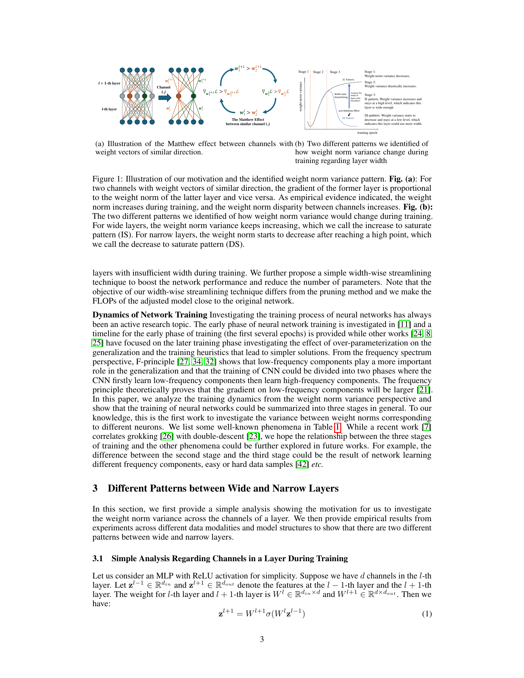
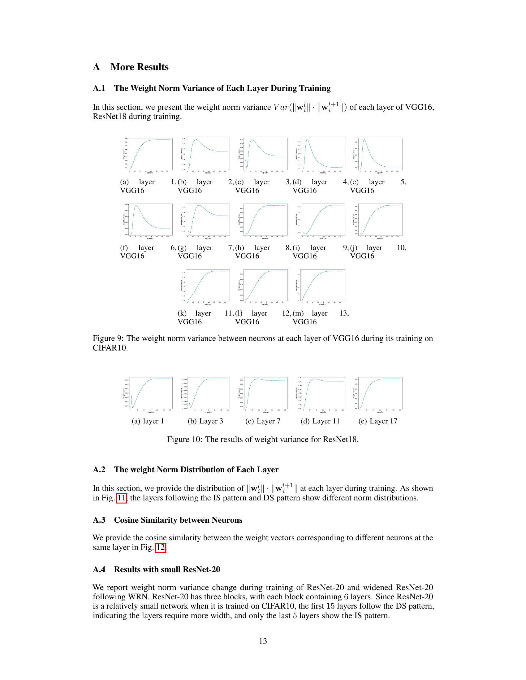
The figure shows the variance of weight norm across different layers of VGG-16 and ResNet18 during training on CIFAR-10. The y-axis represents the variance of weight norm, and the x-axis represents the number of training epochs. Different layers exhibit distinct patterns in weight norm variance change over epochs. The patterns shown are intended to illustrate the difference in variance patterns between wide and narrow layers. The patterns observed across the layers of VGG and ResNet architectures support the paper’s claims regarding the relationship between layer width and weight norm variance.

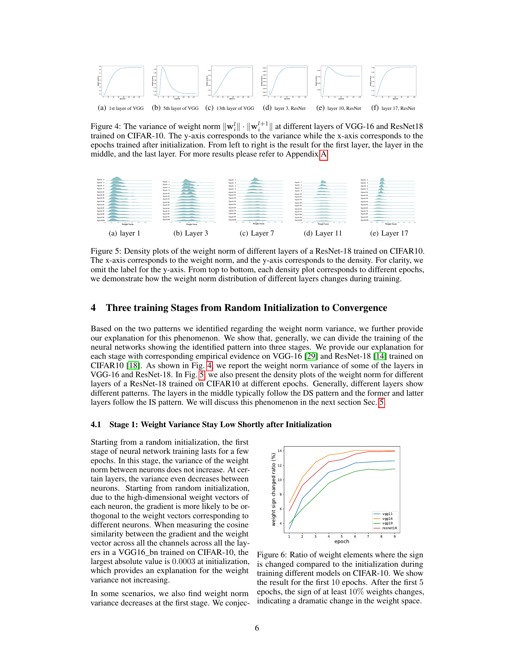
This figure shows the distribution of weight norms for different layers (1, 3, 7, 11, and 17) of a ResNet-18 model trained on CIFAR-10 at various epochs. Each row represents a different epoch, visualizing how the weight norm distribution changes across layers and over time during the training process.

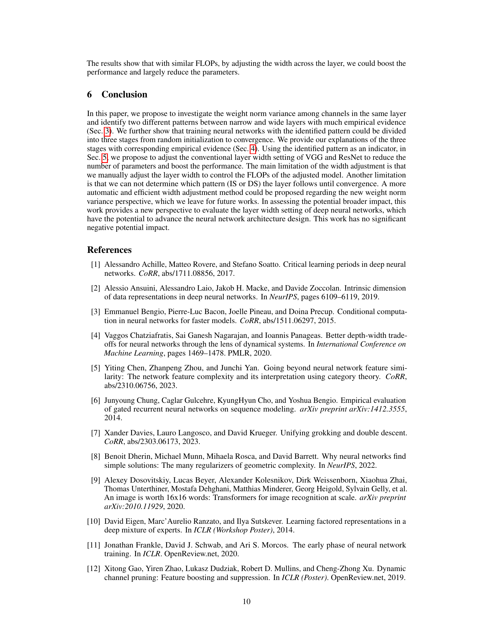
This figure shows the percentage of weight elements that changed sign during the first 10 epochs of training for four different CNN architectures (VGG11, VGG16, VGG19, and ResNet18) on the CIFAR-10 dataset. It demonstrates that a significant portion of weights change sign early in training, highlighting the dynamic nature of the weight space during the initial learning phase. The rapid changes suggest a period of chaotic exploration before the network settles into a more stable solution.

This figure shows the training dynamics of a VGG16 network on the CIFAR-10 dataset. Panel (a) displays the loss, accuracy, and weight norm variance of the 5th layer over 150 epochs. It highlights the rapid performance increase during the second training stage (around epoch 20), correlating with a drastic increase in weight norm variance. Panel (b) demonstrates the strong correlation between weight norm at epoch 6 and the final weight norm, suggesting the early training stages are crucial in determining the final weight distribution.

This figure shows the cosine similarity between weight vectors of neurons in the same layer of a VGG16 network trained on CIFAR-10. Neurons are sorted by weight norm in descending order (highest weight norm at index 0). The heatmaps visualize the cosine similarity between neuron weight vectors. The figure demonstrates how the similarity patterns differ across layers with different training behaviors (IS and DS patterns). The 5th layer, displaying near-orthogonality (values close to 0), is a representative example of the DS pattern; the first and 13th layers show different similarity structures.
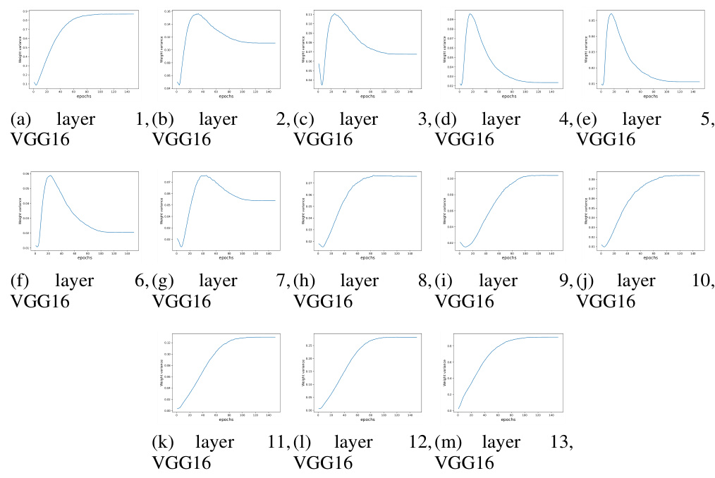
This figure shows the weight norm variance between neurons at each layer of a VGG16 network trained on the CIFAR-10 dataset. Each subplot represents a different layer of the network, and the x-axis shows the training epochs, while the y-axis displays the variance of the weight norms. The plots illustrate how the weight norm variance changes over the course of training for each layer. Analyzing these plots can reveal insights into the training dynamics of each layer and how the width of the layers affects the variance.

This figure shows the distribution of weight norms for different layers (1, 3, 7, 11, 17) of a ResNet-18 model trained on the CIFAR-10 dataset at various training epochs. The x-axis represents the weight norm, and the y-axis represents the density of neurons with that weight norm. The figure illustrates how the weight norm distribution evolves across different layers and training stages.
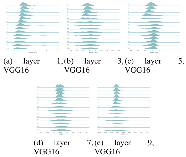
This figure visualizes the distribution of weight norms across different channels within each layer of a VGG16 convolutional neural network trained on the CIFAR-10 dataset. Each subplot represents a different layer of the network. Within each subplot, there are multiple density plots, one for each epoch of training. The x-axis represents the weight norm, and the y-axis represents the density of channels with that particular weight norm. The figure helps illustrate how the distribution of weight norms changes across layers and over the course of training.

This figure visualizes the cosine similarity between weight vectors for different neurons within the same layer of a VGG16 model trained on the CIFAR-10 dataset. Each subplot represents a different layer (1-13). The color intensity in each heatmap indicates the cosine similarity; red represents high similarity, blue represents low similarity, and white represents near-zero similarity. This helps to show how similar the learned features within a layer are. Wide layers might have more neurons with similar weight vectors (redder heatmaps), while narrow layers may show more scattered weight vectors (bluer heatmaps).

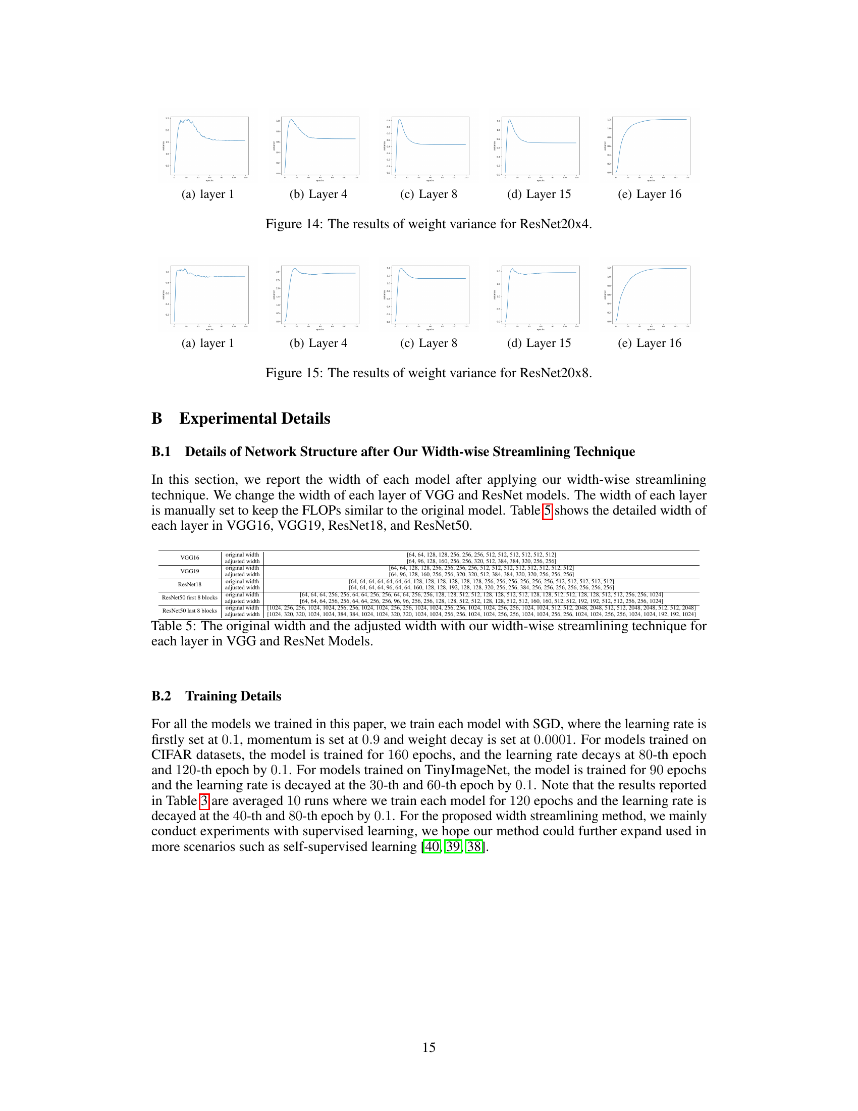
This figure shows the weight norm variance change during the training of ResNet20. Each subplot corresponds to a different layer of the network (Layer 1, Layer 4, Layer 8, Layer 15, Layer 16). The x-axis represents the training epochs, and the y-axis represents the weight variance. The plots illustrate the patterns of weight norm variance changes for different layers during training, showing whether each layer follows an increasing to saturate (IS) pattern or a decreasing to saturate (DS) pattern.

This figure shows the weight norm variance across different channels for each layer (1, 4, 8, 15, 16) of a ResNet20 model during training. Each subplot shows how the variance changes over training epochs. This illustrates the ‘decrease to saturate’ (DS) and ‘increase to saturate’ (IS) patterns observed in narrow and wide layers, respectively. The patterns observed can help determine if a layer is appropriately sized or requires adjustment.

This figure shows the weight norm variance change during training for each layer of a ResNet-20 model. Each subplot represents a layer of the network. The x-axis represents training epochs, and the y-axis represents the weight norm variance. The plot visualizes how the weight norm variance changes over the training process for each layer, illustrating the dynamics of weight distribution learning within the ResNet-20 architecture. This is particularly relevant to the paper’s analysis of wide vs. narrow layers and their distinct training patterns.
More on tables

This table presents the results of applying the IFM (Insufficient Feature Map) algorithm to merge neurons (channels) within layers of a VGG16 model trained on the CIFAR-10 dataset. It compares the original width of each layer to the width after neuron merging using the IFM technique. The final column indicates whether each layer exhibits an ‘IS’ (Increase to Saturate) or ‘DS’ (Decrease to Saturate) pattern of weight norm variance during the third training stage. The IS/DS pattern is an indicator of layer width sufficiency discussed in the paper.

This table presents a comparison of the original and width-adjusted versions of VGG16, VGG19, ResNet18, and ResNet50 models. It shows the number of parameters, FLOPs (floating-point operations), and top-1 accuracy on CIFAR-10 and CIFAR-100 datasets. The width-adjusted models are designed to have similar FLOPs to the original models but with approximately 40% fewer parameters. The results demonstrate the impact of the width adjustment on model efficiency and performance.

This table shows the validation accuracy of original and streamline-width VGG16 and ResNet18 models trained on TinyImageNet dataset. The streamline width models have adjusted width across layers to reduce parameters while maintaining similar FLOPs to the original models. Each result represents an average of 10 independent runs, with each model trained for 90 epochs. More detailed information about training and model configurations is available in Appendix B.

This table presents a comparison of the original VGG and ResNet models with the proposed width-adjusted models. It shows the number of parameters, FLOPs (floating-point operations), and top-1 accuracy for CIFAR-10 and CIFAR-100 datasets. The width-adjusted models aim to reduce parameters while maintaining similar FLOPs to the originals. The results are averaged over 10 runs, each with a different random seed, ensuring robustness. The goal is to show that the adjusted models improve efficiency (fewer parameters) without significant performance loss.
Full paper#
