Graph Neural Flows for Unveiling Systemic Interactions Among Irregularly Sampled Time Series

↗ OpenReview ↗ NeurIPS Homepage ↗ Chat

TL;DR

#

Key Takeaways

#

Why does it matter?

#

This paper is crucial for researchers working with irregularly sampled time series data, offering a novel approach to model systemic interactions and improve forecasting accuracy. It bridges the gap between continuous-time modeling and graph-based methods, opening new avenues for complex system analysis in various domains. The proposed GNeuralFlow model is computationally efficient and provides interpretable results by learning causal relationships between time series.

Visual Insights

#

This figure visually demonstrates the key difference between interacting and non-interacting systems. The left two panels show trajectories for three variables in a system, once with no interaction (A = 0, the zero matrix) and once with interaction (A is a specified adjacency matrix). The same initial conditions are used in both scenarios. The rightmost two panels repeat the experiment, but with different initial conditions. This highlights how the trajectories change significantly in the presence of interaction when different initial conditions are used, whereas there’s no such change in the non-interacting case. This illustrates the impact of systemic interaction on the overall system dynamics.

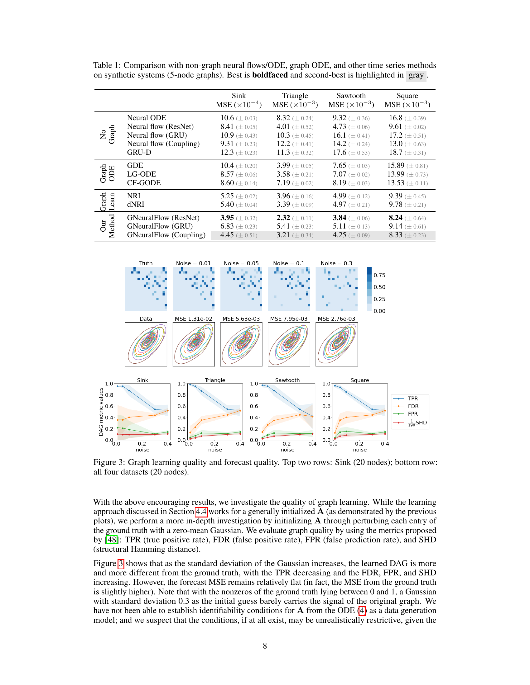
This table presents a comparison of the proposed GNeuralFlow model with various baseline methods on four synthetic time series datasets. The baselines include Neural ODE, neural flows (ResNet, GRU, Coupling), GRU-D, graph ODEs (GDE, LG-ODE, CF-GODE), and graph learning methods (NRI, dNRI). The table shows the Mean Squared Error (MSE) achieved by each method on each dataset. The best performing method for each dataset is shown in boldface, and the second-best method is highlighted in gray. The results demonstrate the superior performance of GNeuralFlow compared to other methods across various graph structures and complexities.

In-depth insights

#

Irregular Time Series

#

Irregular time series data presents unique challenges for analysis and modeling due to the absence of fixed intervals between observations. Traditional time series methods often struggle with such data, leading to inaccurate predictions or a loss of crucial information. Addressing this irregularity is key to improving predictive accuracy and extracting meaningful insights. This requires methodologies that can effectively handle the variable time spacing between data points, possibly through continuous-time modeling or techniques that explicitly model the irregular sampling process. Addressing the impact of missing or irregularly spaced data points is crucial for accurate representation and analysis. Strategies such as imputation, interpolation, or model design that explicitly account for irregular data structures become essential for robust and reliable results. Furthermore, the choice of model greatly affects performance, with some models being inherently more suitable for irregular data than others. Careful consideration of these factors is crucial for uncovering valuable patterns and trends within irregular time series data. Ultimately, handling irregular time series effectively requires innovative techniques and algorithms, and a deep understanding of the underlying data generating process and the chosen modeling approach.

Graph Neural Flows

#

Graph Neural Flows represent a novel approach to modeling complex dynamical systems using time-series data, particularly those with irregular sampling. The core idea involves combining the strengths of neural ordinary differential equations (ODEs) with graph neural networks (GNNs). Neural ODEs provide a continuous-time framework, enabling accurate modeling of systems that evolve smoothly, whereas GNNs capture intricate interdependencies between system components, represented as a graph. The innovative aspect is the integration of a directed acyclic graph (DAG) structure learning into the neural flow model. This DAG explicitly models the conditional dependencies between the time series, thus improving the interpretation and performance of the model. The methodology is shown to outperform traditional methods, offering enhanced efficiency due to bypassing numerical ODE solvers and delivering improved performance in time-series classification and forecasting tasks.

Systemic Interactions

#

The concept of ‘Systemic Interactions’ in a research paper likely refers to the interconnectedness and interdependence of various components within a complex system. A deep analysis would explore how these interactions influence overall system dynamics, going beyond simply observing individual components. Causality is a crucial element, investigating how changes in one part propagate through the system, potentially leading to cascading effects or emergent behavior. The analysis might leverage graph theory to model relationships and dependencies between components, allowing for visualization and quantitative analysis of the interaction network. The paper likely examines the implications of these interactions for prediction and forecasting. Understanding systemic interactions is critical for accurately modeling and managing complex systems, whether biological, social, or technological, as it moves beyond simplistic, reductionist approaches to embrace a holistic view. A robust analysis would also discuss limitations and challenges in identifying and modeling these interactions, particularly in systems with high dimensionality, noisy data, and incomplete information. Novel methods for understanding systemic interactions may be introduced, potentially relying on advanced mathematical or computational techniques. Overall, the section delves into a deeper understanding of system behavior through the lens of interconnectedness.

ODE-Solver-Free

#

The heading ‘ODE-Solver-Free’ highlights a crucial innovation in the paper: eliminating the computational bottleneck of traditional neural ordinary differential equation (NODE) models. NODE models typically rely on iterative numerical solvers to approximate solutions of ordinary differential equations, which can be computationally expensive, especially for long time series or high-dimensional data. The proposed ‘ODE-solver-free’ method directly parameterizes the ODE solution, thereby sidestepping the computationally expensive iterative numerical solver step. This approach provides significant advantages by greatly enhancing computational efficiency and making the model more scalable and practical. It allows the model to handle irregularly sampled time series more effectively, a limitation often found in other graph-based time series analysis models. This efficiency boost is particularly vital for large-scale applications where speed is a critical factor. The core benefit is a more direct and efficient representation, leading to faster training and inference.

DAG-based Modeling

#

DAG-based modeling offers a powerful framework for representing and analyzing complex systems with interconnected components. By representing the system as a directed acyclic graph (DAG), where nodes represent components and edges represent causal relationships or dependencies, we can capture the intricate flow of information and influence. This approach is particularly useful when dealing with scenarios where components interact and influence each other, unlike independent modeling which might miss crucial systemic behaviors. The DAG structure allows for efficient probabilistic modeling, factoring the joint probability distribution into a product of conditional probabilities, thus simplifying the computational complexity. Learning the DAG structure itself is a significant challenge, often requiring specialized algorithms to handle the combinatorial nature of the search space, and often necessitates assumptions about the underlying data generation process. Nonetheless, learned DAGs can provide valuable insights into the system’s causal structure, facilitating improved predictions and more accurate modeling of system dynamics. The effectiveness of DAG-based modeling hinges on the accuracy of the learned DAG and the suitability of the chosen probabilistic model. Inaccuracies in the learned DAG can lead to misleading conclusions and flawed predictions. Careful consideration of these aspects is crucial for successful implementation and interpretation of results.

More visual insights

#

More on figures

This figure compares the performance of neural flows and GNeuralFlow (with both learned and true graphs) on forecasting tasks across four synthetic datasets (Sink, Triangle, Sawtooth, and Square). Each dataset represents a system of interacting time series with a varying number of nodes (3 to 30). The plot shows that GNeuralFlow consistently outperforms standard neural flows in terms of Mean Squared Error (MSE), demonstrating the benefit of incorporating systemic interactions through graph-based modeling.

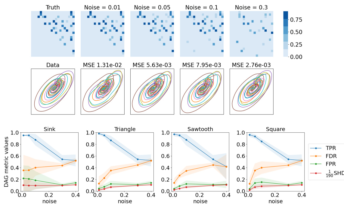
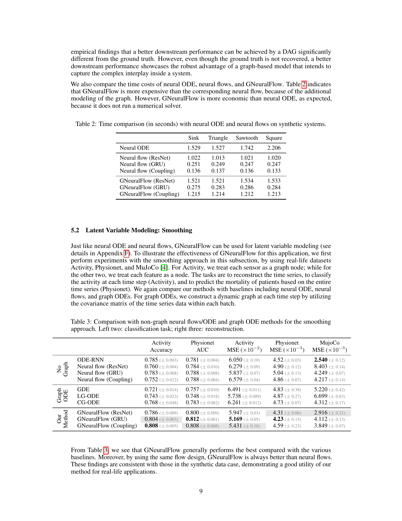
This figure presents the results of graph learning quality and forecast quality. The top two rows show the results for the ‘Sink’ dataset with 20 nodes, demonstrating the effects of varying noise levels on the accuracy of graph learning and forecasting. The bottom row displays a summary of the results across all four datasets (Sink, Triangle, Sawtooth, and Square), providing a comparative analysis of graph learning performance and forecast accuracy under different noise conditions. The metrics used for evaluation are True Positive Rate (TPR), False Discovery Rate (FDR), False Positive Rate (FPR), and Structural Hamming Distance (SHD).

More on tables

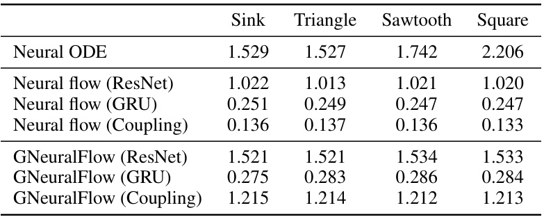
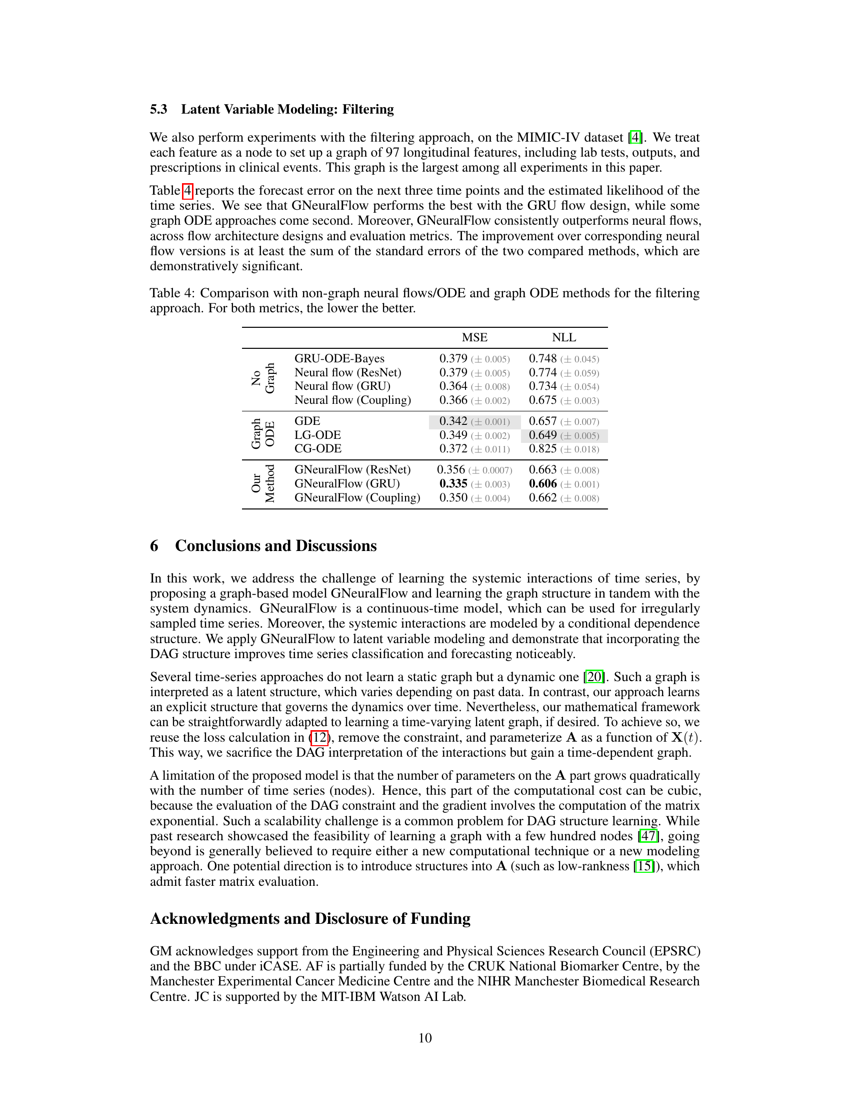
This table compares the computational time (in seconds) taken by Neural ODE, Neural Flows (ResNet, GRU, Coupling), and GNeuralFlow (ResNet, GRU, Coupling) on four different synthetic datasets (Sink, Triangle, Sawtooth, and Square). It demonstrates the relative computational efficiency of each method. GNeuralFlow, while more computationally expensive than the corresponding neural flows, is still more efficient than Neural ODE, which uses numerical ODE solvers. The results highlight the trade-off between model complexity and computational cost.

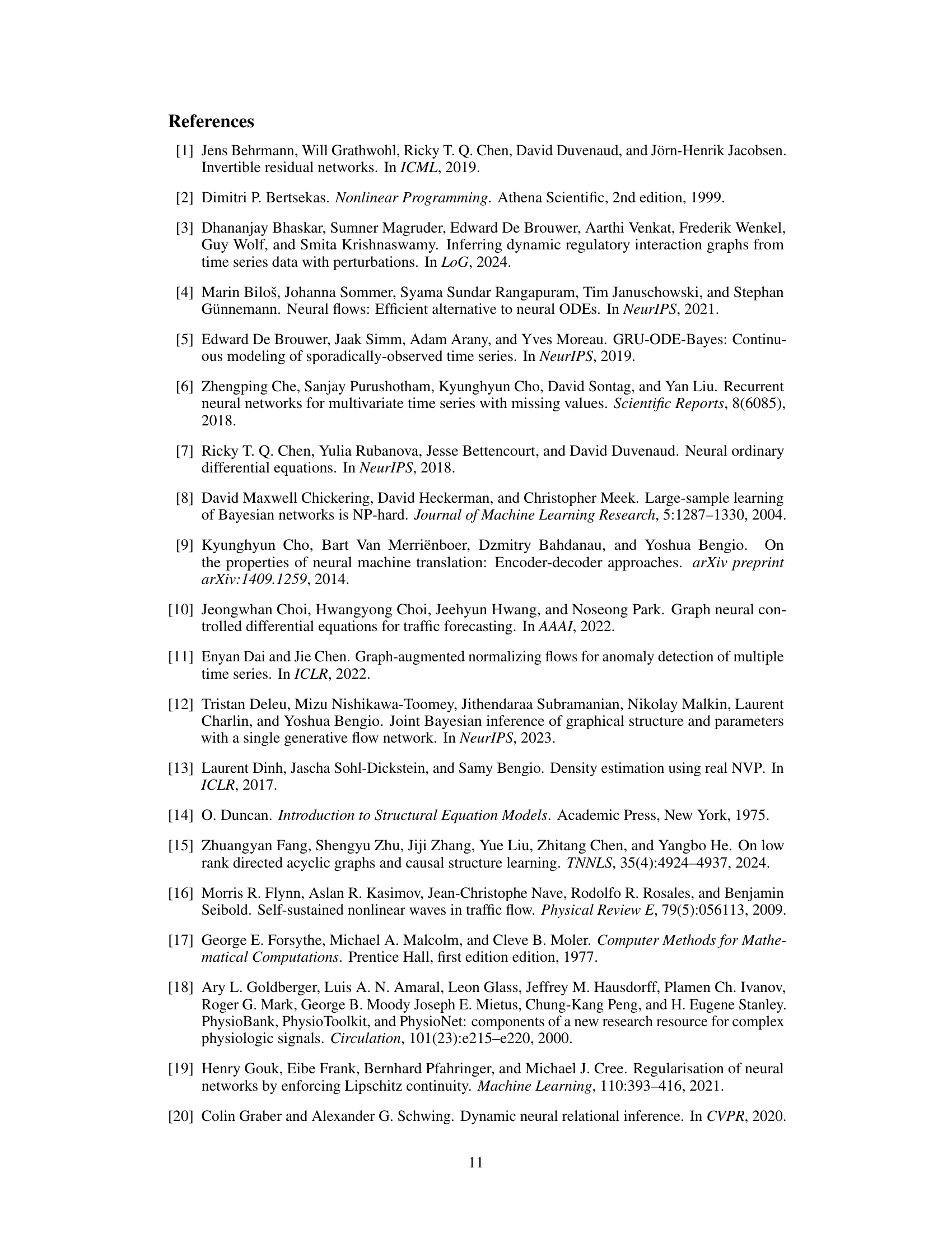
This table presents a comparison of the proposed GNeuralFlow model with several baseline methods on four synthetic time series datasets. Each dataset represents a system of interacting time series with a known graph structure. The table shows the Mean Squared Error (MSE) achieved by each method on the forecasting task, broken down by dataset. The best performing method for each dataset is bolded, and the second-best is highlighted in gray. The methods compared include various neural ODE and flow approaches, along with graph-based ODE methods and other state-of-the-art time series models. The results highlight the superior performance of the proposed GNeuralFlow, demonstrating the benefit of incorporating graph structure and conditional dependencies in the modeling process.

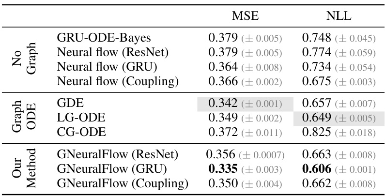
This table compares the performance of GNeuralFlow against various baselines on five synthetic datasets (Sink, Triangle, Sawtooth, and Square) each with a 5-node graph. The metrics used to evaluate the models are Mean Squared Error (MSE). The table highlights the best performing model (boldfaced) and the second-best performing model (in gray) for each dataset. The baselines include Neural ODE, neural flows with different architectures (ResNet, GRU, Coupling), Graph ODE models (GDE, LG-ODE, CF-GODE), and graph learning methods (NRI, dNRI), and non-graph based GRU model (GRU-D). GNeuralFlow is tested with three different architectures (ResNet, GRU, Coupling) as well, demonstrating improved performance across all datasets compared to the baselines.

This table compares the performance of GNeuralFlow against several baseline methods on four synthetic time series datasets. The datasets have 5 nodes in their underlying graph structure. Each model’s Mean Squared Error (MSE) is reported, with the best performance in bold and the second-best highlighted in gray. The baseline methods include traditional neural ODE and neural flow approaches, graph-based ODE models (GDE, LG-ODE, CF-GODE), and other time series models such as NRI and dNRI. The table shows that GNeuralFlow significantly outperforms all baselines on all datasets.

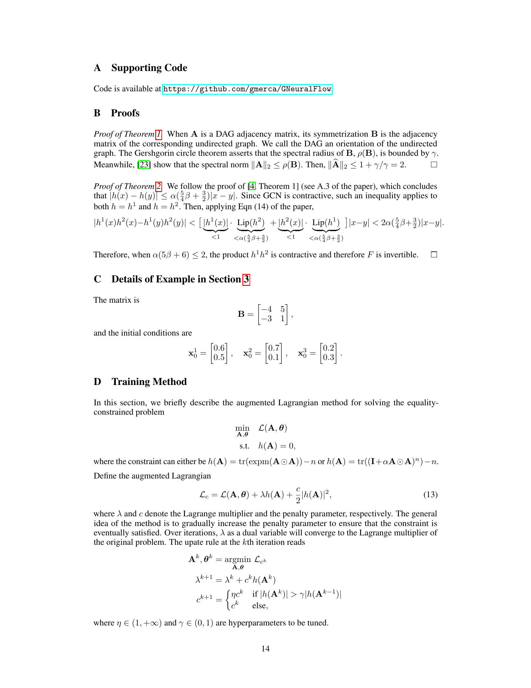
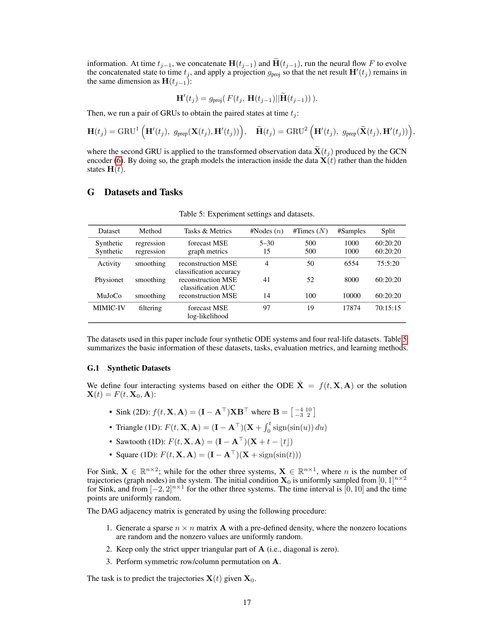
This table summarizes the settings and datasets used in the paper’s experiments. It includes both synthetic and real-life datasets. For each dataset, it specifies the method used (regression or smoothing), the tasks and metrics evaluated, the number of nodes (n), the number of time points (N), the number of samples, and the train/validation/test split.

This table compares the performance of GNeuralFlow against other methods (Neural ODE, neural flows, graph ODEs, graph learning methods, and a non-graph GRU) on four synthetic datasets (Sink, Triangle, Sawtooth, and Square). The results show MSE (Mean Squared Error) for each method. GNeuralFlow consistently outperforms other methods, highlighting the benefits of its graph-based continuous-time approach. The table includes results for various flow architectures within GNeuralFlow and other methods.

Full paper

#