TL;DR#
Temporal link prediction, crucial for various applications, faces challenges in efficient relative encoding construction and limited consideration of temporal information in existing methods. These encodings, usually based on structural connectivity, are computationally expensive and may not fully capture temporal dynamics.
This paper proposes TPNet, a novel temporal graph neural network. TPNet introduces a temporal walk matrix to efficiently incorporate both structural and temporal information, simultaneously considering time decay effects. It leverages random feature propagation, offering theoretical guarantees and improved computation/storage efficiency. TPNet significantly outperforms existing baselines across multiple datasets, achieving a maximum speedup of 33.3x.
Key Takeaways#
Why does it matter?#
This paper is crucial for researchers in temporal link prediction due to its novel approach to relative encoding. It offers a more efficient and effective method, improving upon existing techniques and opening avenues for future research in temporal graph neural networks. Its theoretical guarantees and empirical validation add to its significance.
Visual Insights#

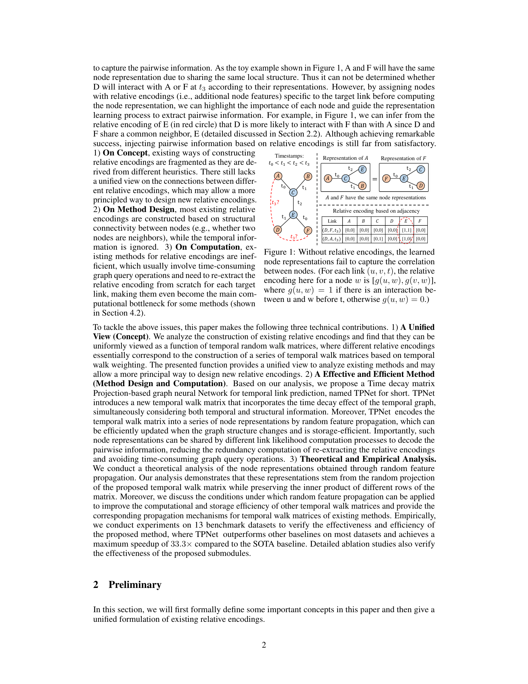
🔼 This figure shows an example of a temporal graph and a temporal walk on that graph. The temporal graph (a) illustrates nodes (A, B, C, D, F) and their interactions with timestamps (t1, t2, t3, t4). The temporal walk (b) highlights a specific sequence of nodes visited [(B, t), (C, t₄), (A, t3), (D, t2), (F, t₁)] with decreasing timestamps, illustrating how the concept of temporal walk relates to the evolution of the temporal graph.
read the caption
Figure 2: A illustration of the temporal walk.
🔼 This table presents the performance comparison of TPNet against 11 other baselines on 13 benchmark datasets for the transductive setting using random negative sampling. The metrics used are Average Precision (AP) and Area Under the Receiver Operating Characteristic Curve (AUC). The results show TPNet’s superior performance on most datasets.
read the caption
Table 1: Transductive results for different baselines under the random negative sampling strategy.
In-depth insights#
Temporal Encoding#
Temporal encoding in temporal link prediction aims to capture the crucial temporal dynamics within interactions. Effective methods must go beyond simply considering timestamps, instead focusing on relative timestamps and the temporal order of events. Representations need to encode relationships between nodes not only based on their adjacency, but also on their temporal proximity and the sequence of interactions. This is challenging because efficient computation of such encodings is essential for scalability. Approaches like using temporal walk matrices offer a systematic way to consider both structural and temporal information but maintaining these matrices efficiently is a key concern. Therefore, innovative techniques are necessary to generate and manage these temporal encodings, such as random feature propagation or other efficient approximation methods, all while ensuring that the temporal information is adequately preserved for accurate predictions.
TPNet Architecture#
TPNet’s architecture is likely composed of two main modules: Node Representation Maintaining (NRM) and Link Likelihood Computing (LLC). NRM focuses on encoding pairwise information by maintaining a series of node representations, efficiently updated upon new interactions via a random feature propagation mechanism. This mechanism implicitly maintains temporal walk matrices, improving computational efficiency. The LLC module then uses these refined node representations and auxiliary features (e.g., link features) to compute the likelihood of a predicted link. A key innovation is the use of a novel temporal walk matrix incorporating time decay, enabling the simultaneous consideration of temporal and structural information. The random feature propagation is theoretically grounded, offering guarantees on the preservation of essential information within the compressed representation. This design thus prioritizes efficiency without sacrificing accuracy by avoiding explicit storage and computation of large temporal walk matrices.
Random Feature#
The concept of “random feature” in machine learning, particularly within the context of a research paper focusing on temporal link prediction, is a powerful technique for dimensionality reduction and efficient computation. Random projections, where data is transformed using a random matrix, are at the core of this approach. This allows for the creation of lower-dimensional feature vectors that approximately preserve the essential information of the higher-dimensional space. This is beneficial because in temporal graph analysis, dealing with potentially huge matrices of temporal walks becomes computationally expensive. Random feature propagation leverages this to maintain the relevant temporal information implicitly through updating compressed node representations as interactions occur. This offers both substantial speedup and reduced memory footprint compared to explicitly storing and manipulating the full matrices. The effectiveness of this strategy relies on theoretical guarantees that prove the approximate preservation of inner products between the original feature vectors in the lower-dimensional space. This approach is not without limitations, as the dimensionality of the random features needs careful consideration to balance the trade-off between accuracy and efficiency, but it presents a viable and innovative solution for addressing the computational challenges inherent in temporal graph analytics.
Efficiency Analysis#
An efficiency analysis in a research paper is crucial for demonstrating the practical applicability of proposed methods. It should go beyond simply stating speed improvements and delve into a nuanced comparison with existing approaches. A strong analysis will quantify the speedup relative to state-of-the-art baselines, ideally across multiple datasets to show consistency. Detailed breakdowns of computational costs for different components of the algorithm are insightful; identifying bottlenecks and explaining algorithmic choices that mitigate them enhances the analysis. Theoretical guarantees supporting efficiency claims should also be included, providing mathematical justification. The analysis must acknowledge and account for any limitations, such as variations in dataset sizes or computational resources used, thereby ensuring the results are reliable and trustworthy. Finally, the analysis should clearly link efficiency gains to the practical impact, explaining how improvements translate to reduced resource consumption or faster processing times for real-world applications.
Future Works#
The paper’s ‘Future Works’ section could explore several promising avenues. Extending TPNet to handle diverse data modalities beyond graph structure and timestamps (e.g., incorporating text or image data) is crucial to broaden applicability. Developing more sophisticated time decay functions that adapt dynamically to varying data patterns could greatly enhance the model’s robustness. Investigating the theoretical underpinnings of random feature propagation for different temporal walk matrices to identify optimal conditions would improve efficiency and generalization. Finally, a detailed comparative analysis against a broader range of baselines, particularly those using advanced attention mechanisms and transformer architectures, is warranted to fully establish TPNet’s performance advantages.
More visual insights#
More on figures

🔼 The figure illustrates a temporal graph and a temporal walk on that graph. The temporal graph (a) shows nodes and edges with timestamps, representing interactions among entities over time. The temporal walk (b) highlights a specific sequence of node-time pairs, demonstrating a path through the graph where the timestamps decrease along the sequence. This path respects the temporal order of interactions.
read the caption
Figure 2: A illustration of the temporal walk.

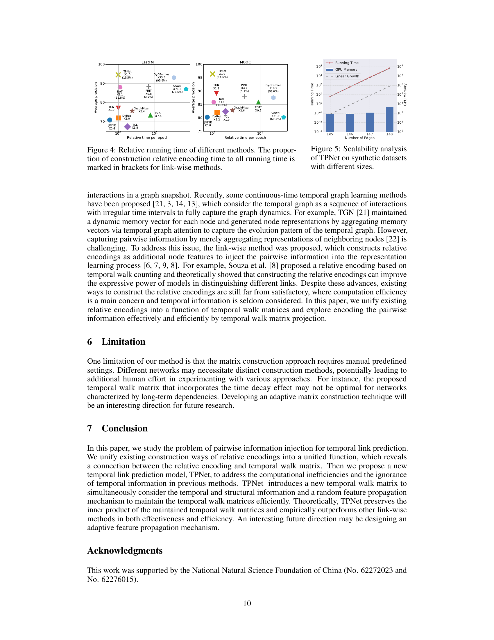
🔼 The plots show the influence of node representation dimension on the average precision of TPNet-d and the SOTA baseline on LastFM and MOOC datasets. The x-axis represents the log2 of the node representation dimension, and the y-axis represents the average precision. It demonstrates the impact of the dimension on model performance.
read the caption
Figure 3: Influence of node representation dimension.
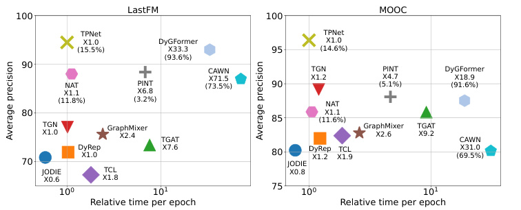
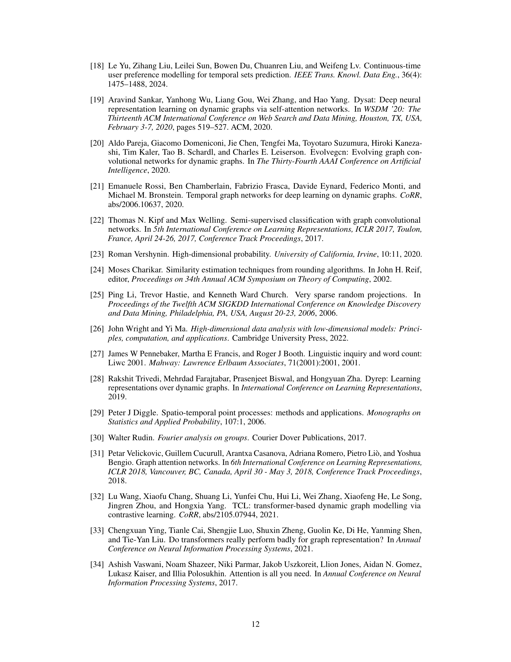
🔼 This figure compares the relative inference time of different methods on two datasets (LastFM and MOOC). It demonstrates that TPNet is significantly faster than other link-wise methods (CAWN, NAT, PINT, DyGFormer) and comparable to node-wise methods. The figure highlights TPNet’s efficiency gains due to its optimized method for maintaining temporal walk matrices, avoiding redundant computations associated with existing methods.
read the caption
Figure 4: Relative running time of different methods. The proportion of construction relative encoding time to all running time is marked in brackets for link-wise methods.
🔼 This figure compares the relative inference time of different methods to TPNet, evaluating their efficiency. The results on LastFM and MOOC datasets are shown. TPNet achieves superior performance and efficiency compared to other methods, particularly link-wise methods which are significantly slower due to the time-consuming relative encoding construction. The figure visually highlights TPNet’s speed advantage, showcasing its efficiency gains.
read the caption
Figure 4: Relative running time of different methods. The proportion of construction relative encoding time to all running time is marked in brackets for link-wise methods.

🔼 This figure illustrates a temporal graph and a temporal walk on it. The temporal graph (a) shows nodes with timestamps indicating interactions over time. The temporal walk (b) highlights a specific path in the graph, demonstrating the concept of a sequence of node-time pairs with decreasing timestamps. This concept is important for understanding temporal link prediction, as it shows how past interactions contribute to predicting future links. The temporal walk helps capture both structural information (connectivity of nodes) and temporal information (order of interactions).
read the caption
Figure 2: A illustration of the temporal walk.

🔼 This figure shows an example temporal graph with nodes and edges. It also illustrates a temporal walk, which is a sequence of nodes visited in decreasing order of timestamps. The temporal walk shown is [(B, t4), (C, t4), (A, t3), (D, t2), (F, t1)]. This example visually explains the concept of a temporal walk which is crucial to the TPNet model.
read the caption
Figure 2: A illustration of the temporal walk.

🔼 The figure contains two parts. Part (a) shows an example of a temporal graph with nodes and edges associated with timestamps. Part (b) shows a temporal walk, which is a sequence of node-time pairs with decreasing timestamps. The example shows a temporal walk with five nodes and their timestamps.
read the caption
Figure 2: A illustration of the temporal walk.

🔼 The plots show how the average precision changes with different node representation dimensions on three datasets (LastFM, MOOC, and Enron). The results demonstrate that a relatively small dimension of node representation can achieve satisfactory performance, indicating the effectiveness and efficiency of TPNet’s random feature propagation mechanism.
read the caption
Figure 3: Influence of node representation dimension.
More on tables
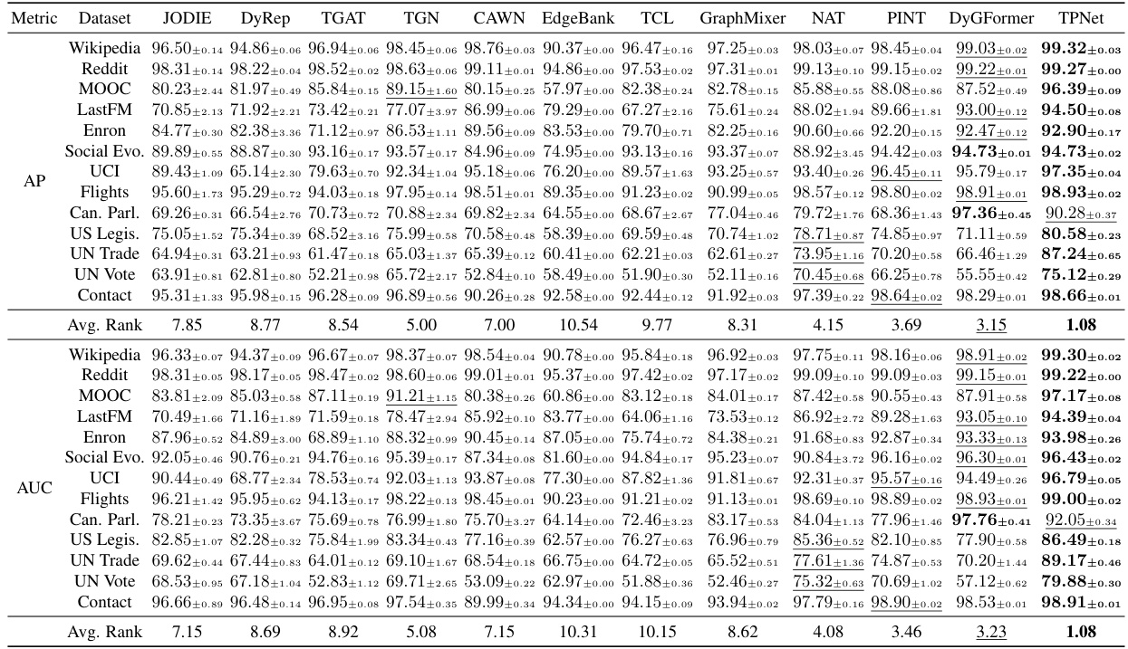
🔼 This table presents the results of a temporal link prediction experiment using various baselines on 13 benchmark datasets under the transductive setting and random negative sampling strategy. The table shows the average precision (AP) and area under the receiver operating characteristic curve (AUC) for each baseline and dataset. The best and second-best results for each dataset are highlighted.
read the caption
Table 1: Transductive results for different baselines under the random negative sampling strategy. blod and underline highlight the best and second best result respectively.
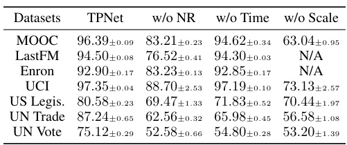
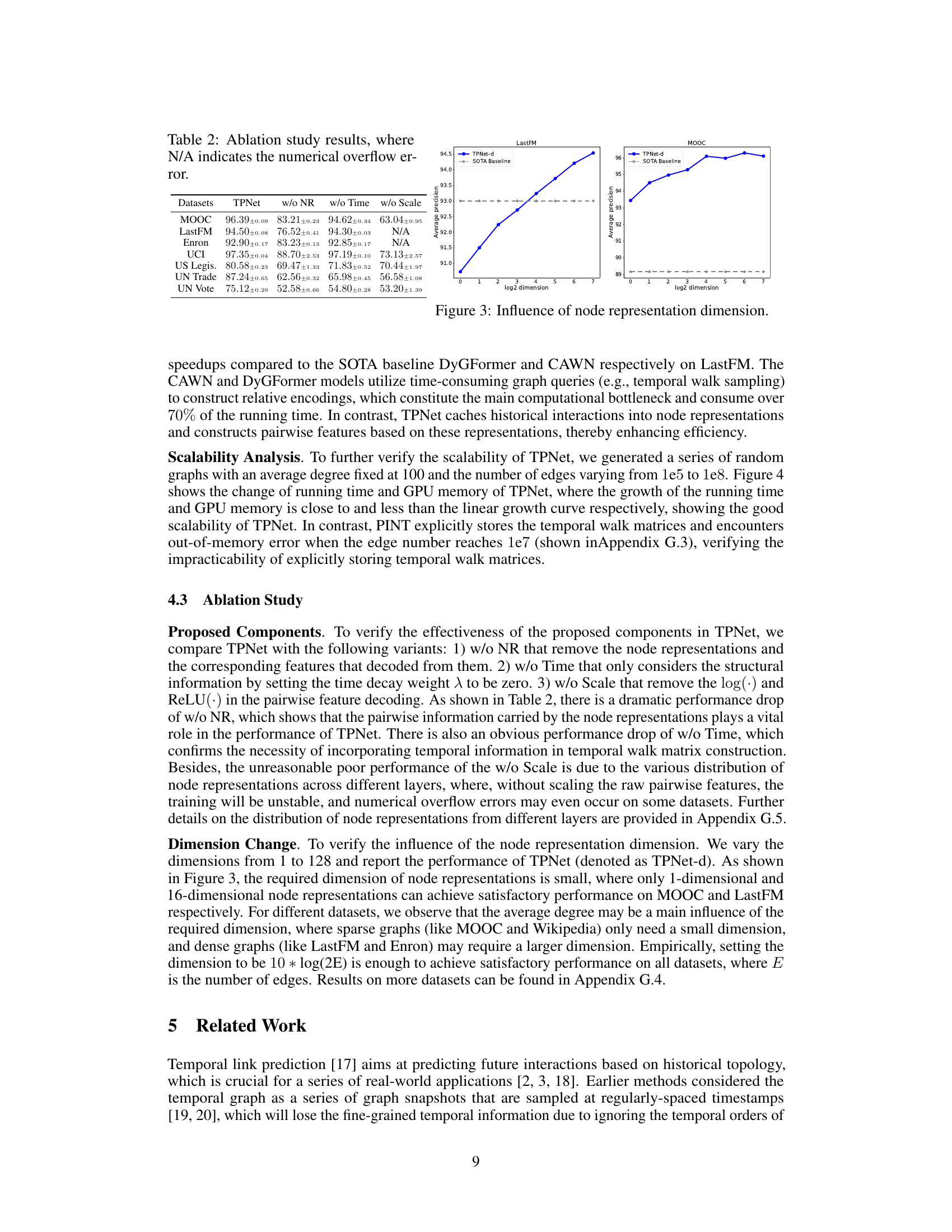
🔼 This table presents the ablation study results, comparing the performance of the TPNet model with different components removed. It shows the impact of removing the node representation maintaining (NRM) module, ignoring the time decay effect in the temporal walk matrix, and removing the scaling and ReLU operations in the pairwise feature decoding. The results demonstrate the importance of each component in achieving high prediction accuracy, particularly highlighting the critical role of the NRM and the time decay effect.
read the caption
Table 2: Ablation study results, where N/A indicates the numerical overflow error.
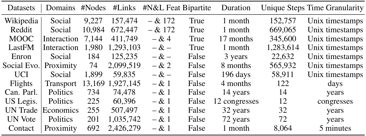
🔼 This table provides a detailed overview of the thirteen benchmark datasets used in the paper’s experiments. For each dataset, it lists the domain, number of nodes and links, the dimensionality of node and link features, whether it is a bipartite graph, the duration of data collection, the number of unique time steps, and the time granularity.
read the caption
Table 3: Statistics of the datasets.

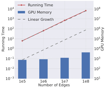
🔼 This table shows the scalability results of the PINT model on synthetic datasets with varying numbers of edges. The ‘Time’ column represents the running time in seconds, and the ‘Memory’ column represents the memory usage in GB. As the number of edges increases, the running time and memory usage increase significantly. At 10,000,000 and 100,000,000 edges, the model runs out of memory (OOM). This highlights a significant limitation of the PINT model’s approach to handling large-scale temporal graphs.
read the caption
Table 4: Scalability analysis of PINT.
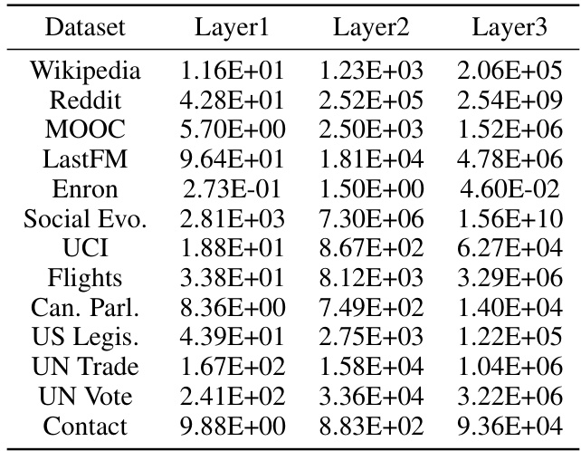
🔼 This table presents a statistical overview of the node representation norms across different layers (Layer1, Layer2, Layer3) for thirteen distinct datasets. Each entry represents the average norm (L2 norm) calculated for the node representations within that specific layer and dataset. The data provides insight into the magnitude and distribution of learned node features at different layers of the TPNet model.
read the caption
Table 5: Average norm of node representations from different layers.
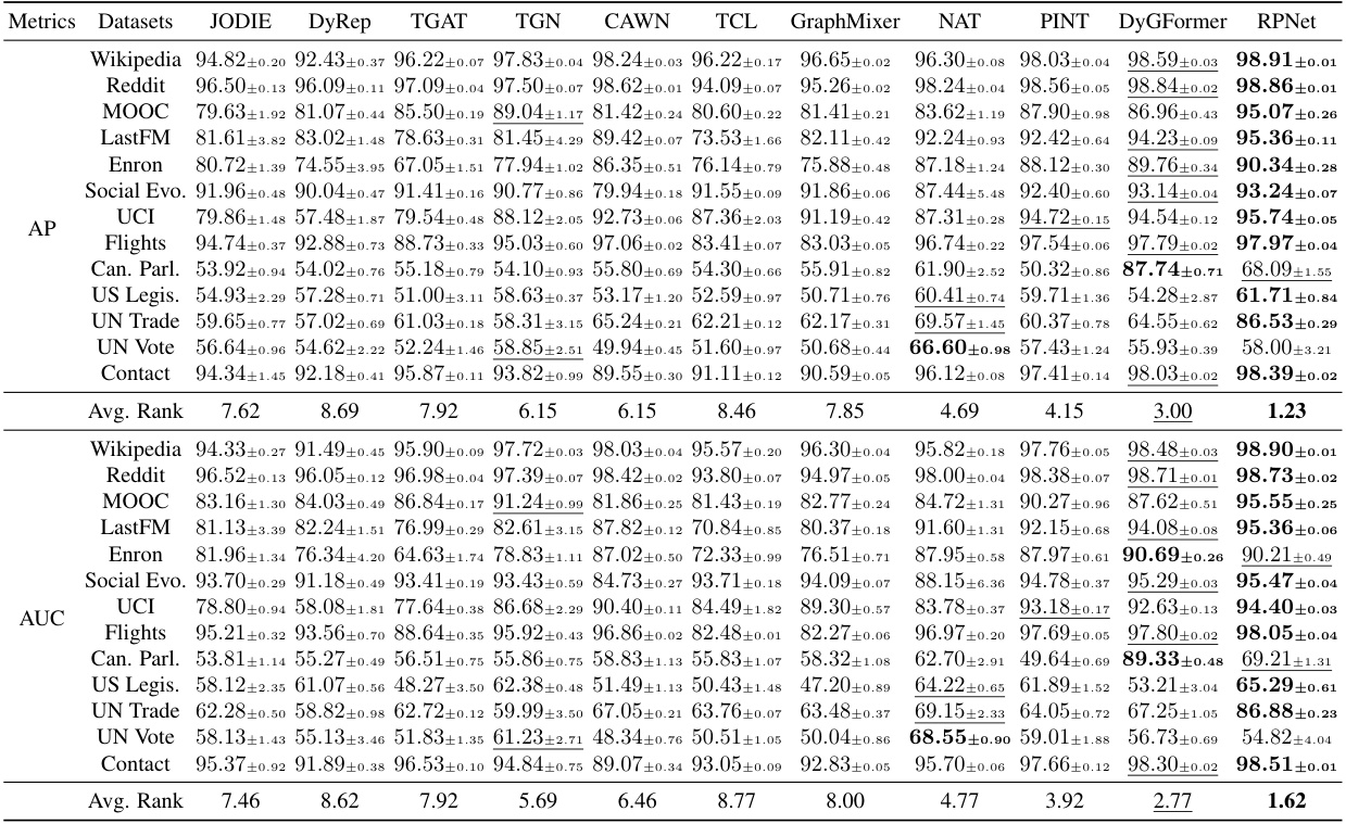
🔼 This table presents the performance comparison of TPNet against 11 other baselines on 13 benchmark datasets for temporal link prediction using the random negative sampling strategy in a transductive setting. The results show the average precision (AP) and area under the receiver operating characteristic curve (AUC) for each method on each dataset. It highlights the effectiveness of TPNet by comparing its performance to the state-of-the-art (SOTA) methods.
read the caption
Table 1: Transductive results for different baselines under the random negative sampling strategy.
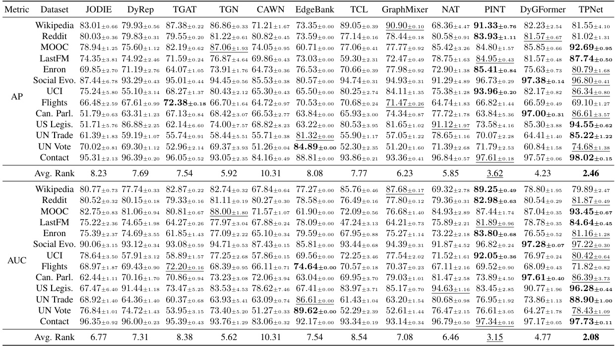
🔼 This table presents the performance comparison of TPNet against 11 other baselines across 13 benchmark datasets. The experiments are conducted under the transductive setting using the random negative sampling strategy. The results are reported as Average Precision (AP). The best-performing model for each dataset is highlighted.
read the caption
Table 1: Transductive results for different baselines under the random negative sampling strategy.

🔼 This table presents the results of a transductive learning experiment on 13 benchmark datasets. The experiment evaluates the performance of 12 different baselines and TPNet (the proposed model) on the task of temporal link prediction. The performance metric is Average Precision (AP) and Area Under the ROC Curve (AUC). Each row represents the results for a specific dataset, and the columns represent the different methods evaluated. The best and second-best results for each dataset are highlighted in bold and underlined, respectively. This table demonstrates TPNet’s superior performance compared to the baseline methods across various datasets.
read the caption
Table 1: Transductive results for different baselines under the random negative sampling strategy. blod and underline highlight the best and second best result respectively.

🔼 This table presents the performance comparison of TPNet against 11 other baselines on 13 benchmark datasets. The results are for the transductive setting (where the model has seen all nodes and edges during training) and uses a random negative sampling strategy to generate negative samples. The metrics used to evaluate the performance are Average Precision (AP) and Area Under the Receiver Operating Characteristic Curve (AUC). The table highlights the effectiveness of TPNet compared to other methods by showing its superior performance in most datasets.
read the caption
Table 1: Transductive results for different baselines under the random negative sampling strategy.

🔼 This table presents the performance of TPNet and other baselines on 13 benchmark datasets for temporal link prediction. The results are reported using Average Precision (AP) and Area Under the Receiver Operating Characteristic Curve (AUC-ROC) metrics. The table demonstrates TPNet’s superior performance compared to the other methods, showcasing its effectiveness in capturing both temporal and structural correlations in dynamic graph data.
read the caption
Table 1: Transductive results for different baselines under the random negative sampling strategy.
Full paper#
