Dynamic Conditional Optimal Transport through Simulation-Free Flows

↗ OpenReview ↗ NeurIPS Homepage ↗ Chat

TL;DR

#

Key Takeaways

#

Why does it matter?

#

This paper is crucial for researchers working on conditional generative modeling and Bayesian inverse problems. It offers a novel, simulation-free approach that is scalable to high-dimensional and infinite-dimensional settings, directly addressing limitations of existing methods. The dynamic formulation of conditional optimal transport provides a strong theoretical foundation and opens new avenues for developing efficient and principled likelihood-free inference techniques.

Visual Insights

#

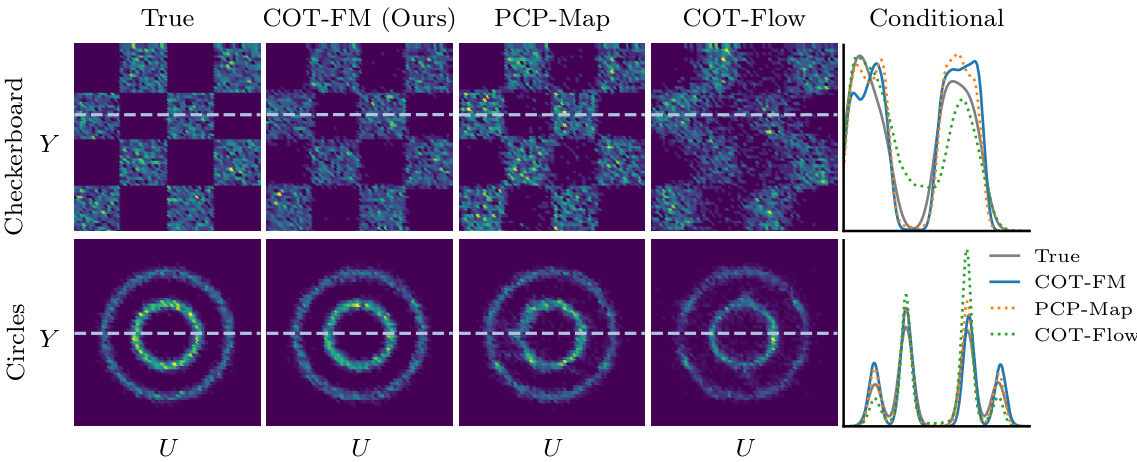
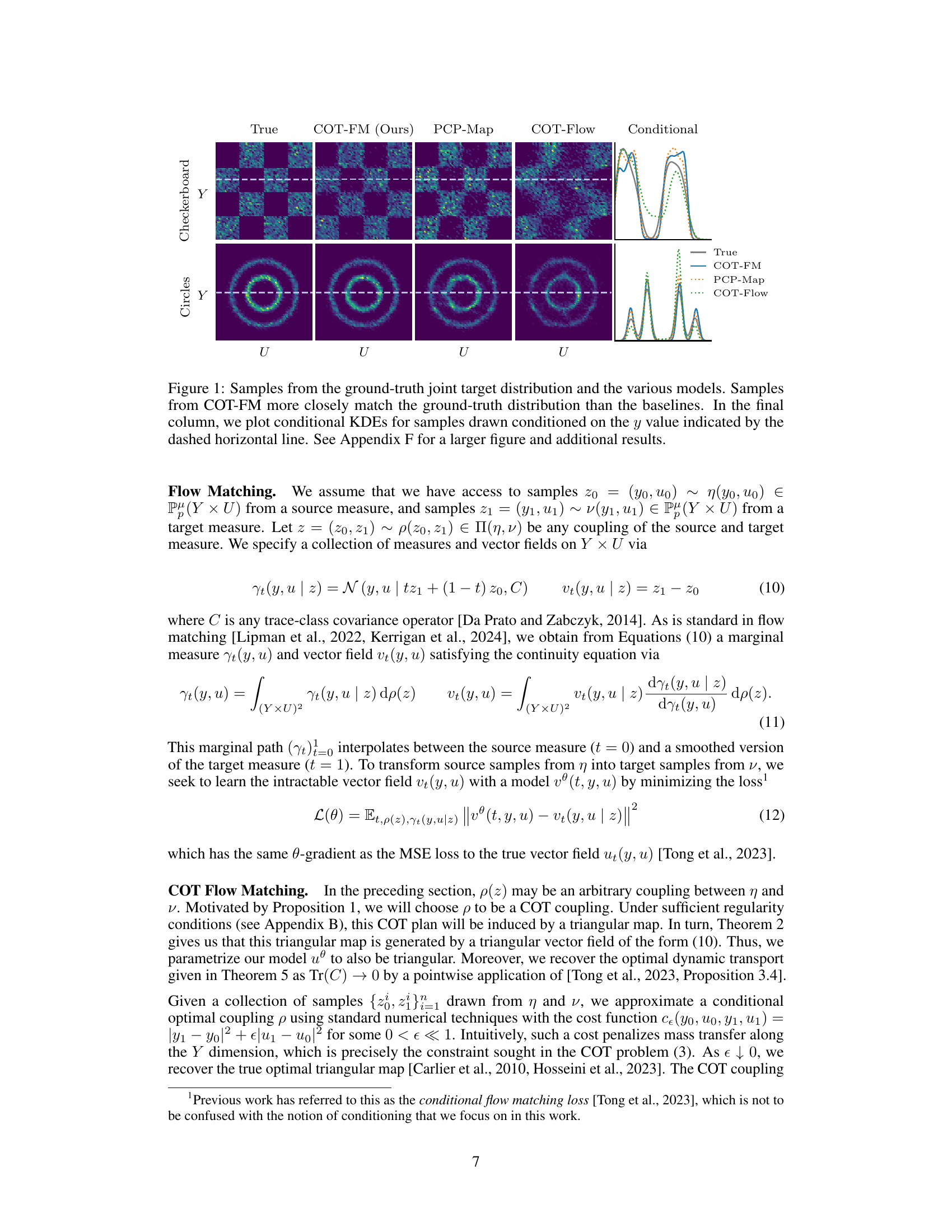
This figure compares samples generated from different conditional generative models against the ground truth. The models shown are COT-FM (the authors’ proposed model), PCP-Map, COT-Flow, and a conditional model. The figure visually demonstrates that COT-FM generates samples that are much closer to the true distribution than the other models, particularly evident in the conditional KDE plots shown for a specific y value.

This table presents the performance comparison of different models on four 2D synthetic datasets (Checkerboard, Moons, Circles, Swissroll). The performance is measured using two metrics: 2-Wasserstein distance (W2) and Maximum Mean Discrepancy (MMD). The results are averaged over five test sets, and the standard deviations are shown. COT-FM consistently achieves lower distances compared to the baselines (PCP-Map, COT-Flow, and FM).

In-depth insights

#

COT Flow Matching

#

The proposed “COT Flow Matching” method cleverly integrates conditional optimal transport (COT) with flow-based generative models. Instead of relying on adversarial training or computationally expensive sampling, it directly learns the geodesic path connecting source and target distributions in the conditional Wasserstein space. This is achieved by using a dynamic formulation of COT, characterized by a continuity equation solved via a triangular vector field. The method’s simulation-free nature is a significant advantage, particularly for high-dimensional or likelihood-free inference problems. By learning this dynamic mapping, new samples are generated by following the learned flow, effectively amortizing the computational cost across different conditions. The theoretical foundation is rigorous, generalizing classic results like the Benamou-Brenier theorem to the conditional setting, and offering a principled approach for challenging tasks like Bayesian inverse problems. The empirical evaluations demonstrate strong results, particularly in high dimensional spaces, indicating the method’s practical usefulness.

Dynamic COT Theory

#

A hypothetical “Dynamic COT Theory” would extend the existing framework of Conditional Optimal Transport (COT) by introducing a temporal dimension. Instead of focusing solely on static mappings between conditional distributions, a dynamic approach would model the evolution of these distributions over time. This could involve studying the geodesics (shortest paths) in a space of conditional measures, potentially using techniques like the Benamou-Brenier theorem to represent transport as a fluid flow. Key research questions would revolve around characterizing the properties of these dynamic geodesics, such as their existence, uniqueness, and stability. Developing efficient algorithms for learning and simulating these dynamic transport plans would be a crucial aspect. Applications could encompass various domains, including Bayesian inverse problems where time-varying data or systems are involved, or in generative modeling where dynamic transitions between conditional distributions are desired. The challenges would include designing loss functions compatible with dynamic COT and ensuring that the models capture the intricate relationships across both time and conditional variables. The practical success of a dynamic COT framework would hinge on developing efficient and scalable computational methods.

Hilbert Space COT

#

The concept of “Hilbert Space COT” suggests an extension of Conditional Optimal Transport (COT) to infinite-dimensional spaces, specifically Hilbert spaces. This is a significant advance because many real-world problems, especially in machine learning and scientific computing, involve data that naturally resides in infinite-dimensional function spaces. Standard COT methods, designed for finite-dimensional spaces, often fail to generalize effectively to these higher-dimensional settings. A Hilbert space COT framework would likely leverage the rich mathematical structure of Hilbert spaces, such as inner products and orthonormal bases, to develop efficient and theoretically sound algorithms for conditional generative modeling and Bayesian inference. Key challenges in developing a Hilbert Space COT framework include defining appropriate probability measures and metrics in the infinite-dimensional space, carefully handling the complexity of infinite-dimensional transport plans, and designing computationally tractable algorithms for solving the related optimization problems. Successful development of such a framework could provide significant improvements in various applications, such as solving Bayesian inverse problems and building more powerful generative models that handle complex functional data.

Simulation-Free Flows

#

The concept of “Simulation-Free Flows” in the context of this research paper likely refers to a novel method for generative modeling that avoids computationally expensive simulations, a common bottleneck in many existing approaches like Markov Chain Monte Carlo (MCMC). The core idea revolves around leveraging the mathematical framework of optimal transport (OT) to directly learn a transformation (a “flow”) between a simple source distribution and a complex target distribution, without the need to repeatedly sample from complex models. This bypasses the need for simulation, thus offering a computationally efficient solution, particularly beneficial for high-dimensional problems or those with expensive likelihood evaluations. The method likely relies on a clever mathematical formulation and efficient algorithmic implementations to achieve this simulation-free process, emphasizing the geometric properties of OT and possibly incorporating techniques such as flow matching. A key advantage is the potential for application in challenging scenarios like Bayesian inverse problems where simulations are prohibitively costly, making it a significant advancement in likelihood-free inference. The paper likely presents both theoretical underpinnings and empirical results demonstrating this method’s competitive performance against traditional simulation-based approaches, particularly in scalability and efficiency.

Inverse Problem App.

#

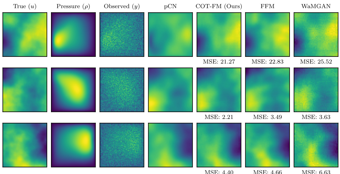
The heading ‘Inverse Problem App.’ suggests a section detailing applications of the research to inverse problems. Inverse problems involve inferring unobservable causes from observed effects, often requiring complex models and challenging computational methods. This section likely showcases the method’s efficacy on such problems, potentially highlighting its ability to handle high-dimensional data, function spaces, or uncertainties which are common features in many real-world inverse problems. The applications could range from scientific simulations (e.g., Darcy flow) requiring expensive numerical solvers to Bayesian inference scenarios in various fields. A successful demonstration in this section would bolster the paper’s claim of practical utility by showing how the core methodology can tackle difficult, relevant problems and outperform existing approaches. The results likely include quantitative metrics assessing performance, comparisons with other methods, and possibly discussion of the model’s limitations in specific application contexts.

More visual insights

#

More on figures

The figure compares samples from four different models against the ground truth for two different 2D datasets. Each model generates samples from a joint distribution of y and u, where y is a condition and u is the unknown to be generated. Visually, COT-FM (the proposed method) shows a better match to the ground truth. The conditional KDE plots provide a quantitative comparison for a fixed condition y.

This figure compares samples generated from the proposed COT-FM model and three baseline methods (PCP-Map, COT-Flow, and Conditional Flow Matching) against the ground truth on three different 2D datasets (Checkerboard, Circles, and Swiss Roll). The figure shows that the COT-FM model produces samples that more closely resemble the ground truth distribution. Conditional KDEs (Kernel Density Estimates) are also included to show the conditional distribution of samples given a specific condition (y-value).

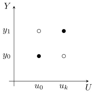
This figure demonstrates a counterexample used in the proof of Proposition 2 in the paper. It visually represents two probability measures, ηk (black dots) and νk (white dots), on a 2D space (Y, U). The measures are constructed to show that there is no constant C such that the conditional Wasserstein distance W(η, ν) is always less than C times the unconditional Wasserstein distance Wp(η, ν) for all measures η and ν. The figure visually illustrates how the conditional Wasserstein distance can grow unboundedly while the unconditional distance remains bounded.

This figure compares samples generated by different models (COT-FM, PCP-Map, COT-Flow, and FM) against the ground truth for four 2D datasets (Checkerboard, Moons, Circles, and Swissroll). The heatmaps visualize the joint distributions, showing that COT-FM produces samples that more closely resemble the ground truth than the other methods. The baselines often fail by generating samples in areas where the true distribution has zero probability.

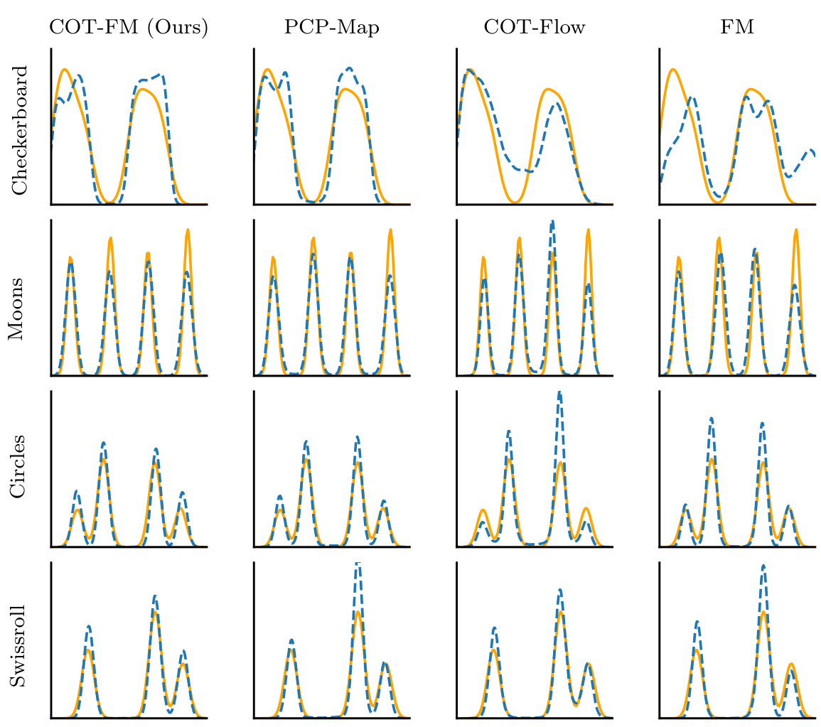
This figure compares the conditional Kernel Density Estimates (KDEs) of the generated samples from four different methods (COT-FM, PCP-Map, COT-Flow, and FM) against the ground truth KDEs on four 2D datasets (Checkerboard, Moons, Circles, and Swissroll). The conditioning variable ‘y’ is held constant at the value indicated by the dashed horizontal line in Figure 5. The plots illustrate how well each method captures the conditional distribution p(u|y).

This figure compares samples generated by different models (COT-FM, PCP-Map, COT-Flow, and Conditional) against the ground truth for two different 2D datasets (Checkerboard and Circles). It shows that the COT-FM model generates samples that are much closer to the ground truth distribution compared to the other three baseline methods. The rightmost column provides a visualization of conditional KDEs, highlighting how well each model captures the conditional distribution given a specific y-value.

This figure compares the performance of different models, including COT-FM (the proposed method), in generating samples from a conditional distribution. The top row shows samples from a checkerboard pattern, while the bottom row shows samples from a circular pattern. The ‘True’ column displays the ground truth, while the other columns represent different models. The final column shows kernel density estimates (KDEs) for each model, given a specific condition (y-value). COT-FM shows the closest match to the ground truth distribution, suggesting superior performance in conditional generation.

This figure compares samples generated from the proposed COT-FM model with those from several baseline models and the ground truth. The samples are visualized using kernel density estimation (KDE) plots for both joint and conditional distributions. The figure demonstrates that COT-FM is able to generate samples closer to the true distribution than baseline models. The conditional KDEs show the ability of the model to generate samples matching the target distribution for a specified condition.

This figure compares samples generated by different models (COT-FM, PCP-Map, COT-Flow, Conditional) against the ground truth for two different datasets (Checkerboard and Circles). It visually demonstrates that the proposed COT-FM method generates samples that better match the true distribution, especially when conditioned on a specific value of y. Conditional KDEs (Kernel Density Estimates) further quantify this difference.

This figure compares samples generated from the proposed COT-FM model against other conditional generative models on several 2D datasets. The figure shows that the COT-FM model generates samples that are visually more similar to the ground truth than the other models. The conditional KDEs further illustrate that the distribution of samples generated by COT-FM is more accurate for a given y value.

This figure compares samples generated from the proposed method (COT-FM) and other baseline methods against the ground truth. The figure shows that COT-FM produces samples that are more similar to the ground truth than those produced by other methods. Conditional KDEs further illustrate the improved performance of COT-FM.

More on tables

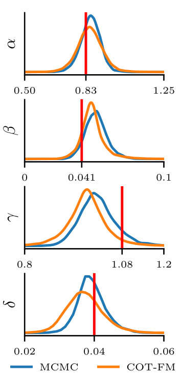
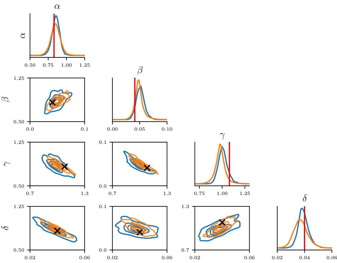
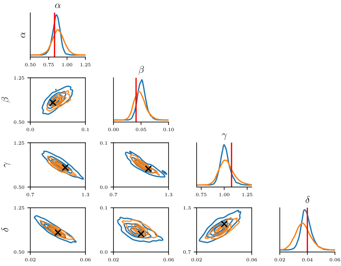
This table presents the results of comparing different methods for estimating the posterior distribution of parameters in a Lotka-Volterra dynamical system. The methods are compared to Markov Chain Monte Carlo (MCMC) using two metrics: the 2-Wasserstein distance and the Maximum Mean Discrepancy (MMD). The table shows that COT-FM achieves the lowest W2 distance, indicating superior performance in capturing the true posterior distribution.

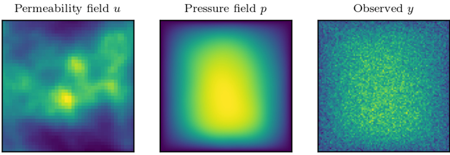
This table presents the mean squared error (MSE) and continuous ranked probability score (CRPS) for the Darcy flow inverse problem. The results are averaged across five test sets, each containing 5,000 samples. Lower MSE and CRPS values indicate better predictive performance.

This table presents a quantitative comparison of the performance of different models on generating samples from four 2D synthetic datasets (checkerboard, moons, circles, swiss roll). The models compared include the proposed method (COT-FM), along with three baselines (PCP-Map, COT-Flow, and FM). The evaluation metrics used are the 2-Wasserstein distance (W2) and the Maximum Mean Discrepancy (MMD). Results are averages across five test sets, reported with standard deviations. COT-FM shows lower distances indicating better performance.

This table presents a quantitative comparison of the performance of different conditional generative models on four 2D synthetic datasets (checkerboard, moons, circles, swiss roll). The models are evaluated using two metrics: the 2-Wasserstein distance (W2) and the Maximum Mean Discrepancy (MMD). The results show that the proposed COT-FM method outperforms other baselines in terms of lower distances to the ground truth distributions.

Full paper

#