↗ OpenReview ↗ NeurIPS Homepage ↗ Chat
TL;DR#
Current methods for learning causal relationships from data using differentiable structure learning often struggle with identifiability issues. The optimizer may exploit undesirable artifacts in the loss function, leading to inconsistent and unreliable results, especially when dealing with multiple global minimizers. Furthermore, existing approaches are sensitive to data scaling, hindering their applicability in real-world scenarios where such transformations are common.
This paper tackles these challenges by introducing a carefully regularized likelihood-based score function. This new score function not only facilitates the use of gradient-based optimization techniques but also possesses key properties. It reliably identifies the sparsest causal model, even in the absence of strong identifiability assumptions, offering more consistent and robust causal discovery. The method is also scale-invariant, ensuring that data standardization does not affect the recovered causal structure, making it more robust to pre-processing decisions.
Key Takeaways#
Why does it matter?#
This paper is crucial because it addresses the critical issue of identifiability and consistency in differentiable structure learning of directed acyclic graphs (DAGs), a fundamental problem in causal inference and machine learning. By proposing a novel likelihood-based score function and proving its ability to recover the sparsest DAG structure, this research significantly advances the field, offering solutions that are both theoretically sound and practically applicable. Furthermore, the scale-invariant property of the proposed score resolves issues encountered by current approaches, paving the way for more robust and reliable causal discovery methods.
Visual Insights#
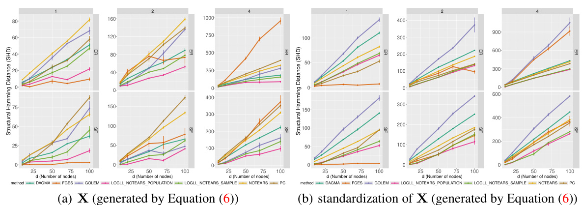
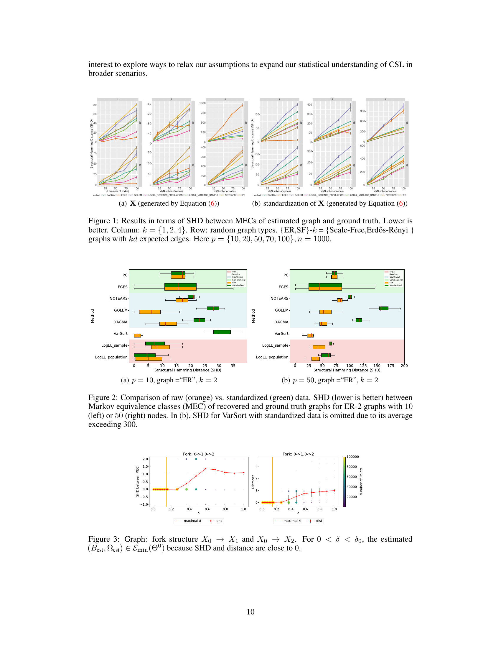
This figure displays the results of structure learning experiments using different methods. The x-axis represents the number of nodes in the graph, and the y-axis represents the structural Hamming distance (SHD) between the estimated graph and the ground truth. A lower SHD indicates better performance. The figure is divided into subplots based on the number of expected edges (k) in the graph, and the type of graph (Erdős-Rényi or Scale-Free). Data is shown for both raw data and standardized data. The results demonstrate how well different algorithms recover causal structure in varying settings.
In-depth insights#
DAGs: A New Score#
A research paper section titled “DAGs: A New Score” would likely introduce a novel scoring function for evaluating the quality of a directed acyclic graph (DAG) structure in causal inference or Bayesian network learning. This new score would ideally address limitations of existing methods, potentially offering improved accuracy, computational efficiency, or robustness to noise or other confounding factors. A key aspect would be a detailed explanation of the score’s mathematical formulation, justifying its properties and relationship to underlying probability distributions. The paper would likely then demonstrate the score’s effectiveness through empirical evaluations on benchmark datasets, comparing its performance against state-of-the-art methods. Theoretical analysis would be crucial, establishing properties such as consistency or asymptotic optimality under certain assumptions. The discussion section might highlight the new score’s advantages and limitations, along with potential avenues for future research, such as extensions to handle different data types or model complexities. Ultimately, the success of this “New Score” hinges on its ability to improve upon existing DAG learning methods, producing superior causal discovery or probabilistic modeling results.
Nonconvex Regularization#
Nonconvex regularization techniques are crucial for addressing challenges in high-dimensional data analysis, particularly within the context of structure learning. Standard convex penalties like L1 often yield biased estimates or fail to recover the true underlying structure effectively. Nonconvex penalties, such as SCAD or MCP, offer a compelling alternative. They combine the desirable sparsity-inducing properties of L1 with improved bias reduction and the ability to identify the true model more accurately. The nonconvexity introduces computational complexity, requiring sophisticated optimization algorithms to guarantee convergence to a global or near-global optimum. However, the theoretical benefits often outweigh the computational cost, especially when dealing with nonidentifiable models where multiple solutions could exist. Careful selection of hyperparameters is critical to balance the benefits of regularization with potential overfitting and numerical stability issues. This nuanced approach enables more accurate and meaningful results compared to traditional convex methods, especially in complex settings where identifying the sparsest or most faithful graph structure is the primary goal.
Scale Invariance#
The concept of scale invariance in the context of causal structure learning is crucial because it ensures that the learned causal relationships are not artifacts of arbitrary scaling or normalization of the data. A scale-invariant method correctly identifies the causal structure regardless of the units of measurement or the range of values used in the dataset. This robustness is vital because real-world data often involves variables measured in different units, and applying a scale-invariant method prevents the discovery of spurious causal relationships resulting from unit inconsistency. The research highlights how the choice of score function significantly impacts scale invariance. While some methods are shown to be susceptible to the units of the variables (e.g., the least squares loss), the study demonstrates that a carefully regularized log-likelihood-based score function possesses the desired scale invariance property. This means that rescaling the variables does not alter the optimal solution of the structure learning task, making the results more reliable and generalizable to real-world scenarios involving various scaling methods.
General Model Results#
A hypothetical ‘General Model Results’ section would likely present empirical evaluations across diverse datasets and model architectures. It would showcase the method’s performance relative to baselines, highlighting strengths and weaknesses. Key metrics, such as precision, recall, F1-score, and AUC, would be reported, potentially with statistical significance tests. The analysis should delve into the model’s behavior under varying conditions, exploring its robustness to noise, sensitivity to hyperparameter choices, and scalability. Visualizations, like boxplots or line graphs, might illuminate the findings. A discussion of any surprising or unexpected results, comparing performance across different data types or complexities, would be vital. A concise summary of the key findings and their implications for the broader field, concluding with future research directions, should complete the section.
Future Research#
Future research directions stemming from this work could explore several promising avenues. Extending the theoretical framework to encompass nonparametric models would enhance the applicability and robustness of the methods. Investigating the impact of different regularizers and their effect on model identifiability and sparsity is crucial. The current approach leverages likelihood-based scoring; exploring alternative scoring functions or hybrid approaches could further refine the methodology and performance. Addressing the computational complexity associated with high-dimensional datasets is another critical aspect. Developing more efficient algorithms or leveraging parallel computing techniques are essential to handle large-scale causal discovery tasks. Finally, incorporating interventional data is a significant challenge and opportunity. Integrating interventions into the model can greatly improve causal inference accuracy and provide a more holistic understanding of causal relationships, which opens a path to further expand the capabilities of this methodology.
More visual insights#
More on figures
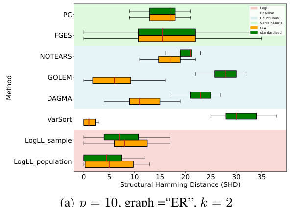
The figure compares the performance of different methods in recovering the true causal structure, represented as a directed acyclic graph (DAG), from data generated by structural equation models (SEMs). The performance is measured using the Structural Hamming Distance (SHD), which quantifies the difference between the estimated DAG and the true DAG. Lower SHD values indicate better accuracy. The figure shows results for different graph types (Erdős-Rényi and Scale-Free) with varying numbers of edges, demonstrating how the methods perform with different levels of sparsity and network structure. It also shows results for different numbers of nodes (p) and sample sizes (n), demonstrating the scalability of the methods. The results suggest that the LOGLL-NOTEARS method performs best overall. The results for the standardized data are shown in (b).
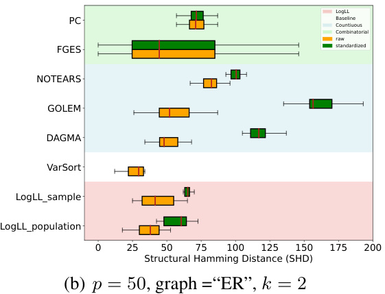
This figure compares the performance of various causal structure learning algorithms on raw and standardized data. The Structural Hamming Distance (SHD) is used to measure the difference between the estimated causal graph structure and the ground truth. Lower SHD values indicate better performance. The figure shows that standardizing the data significantly impacts some algorithms (GOLEM, NOTEARS, DAGMA) causing them to perform much worse compared to using raw data; while others (LOGLL-NOTEARS) maintain robustness to data standardization.

This figure shows the results of an experiment evaluating the impact of the hyperparameter δ on the quality of solutions obtained by the LOGLL-NOTEARS algorithm. The experiment used a simple fork graph structure (X0 → X1 and X0 → X2) and varied δ, while keeping other hyperparameters fixed. The plots show the structural Hamming distance (SHD) between the estimated graph and the true graph, along with the distance between the estimated model parameters and the true parameters. For values of δ less than a certain threshold (δ0), the SHD and distance are both close to zero, indicating that the algorithm successfully recovers the minimal model in the Markov equivalence class. This supports the theoretical findings of the paper which demonstrate that under certain conditions, the LOGLL-NOTEARS algorithm consistently recovers the minimal model within its Markov equivalence class.
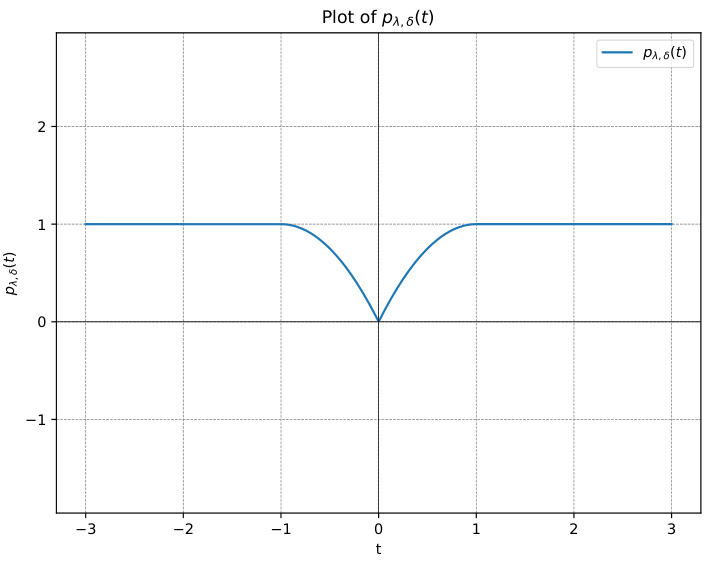
This figure shows a plot of the quasi-MCP penalty function, pλ,δ(t), with parameters λ = 2 and δ = 1. The plot illustrates the function’s behavior: it is constant at 1 for |t| ≥ δ, quadratic for |t| < δ, and smooth throughout its domain. The quasi-MCP penalty combines the properties of a quadratic function near zero, approximating the L2 penalty, with a constant value for larger values of |t|, approximating the L0 penalty. This balance results in a penalty that is both differentiable and encourages sparsity.
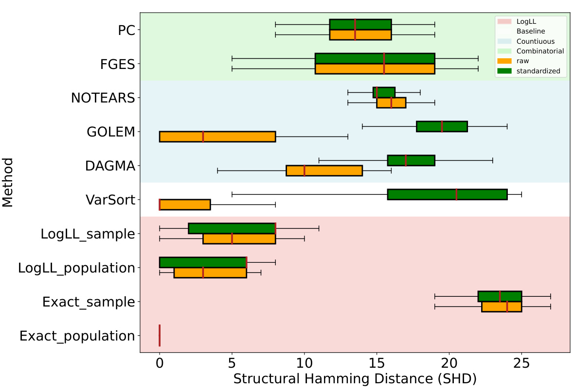
This figure shows the results of the experiment comparing different methods for estimating the structure of directed acyclic graphs (DAGs). The results are evaluated using Structural Hamming Distance (SHD), which measures the difference between the estimated DAG and the true DAG. The experiment varies the number of nodes (p) and edges (k) in the DAG, as well as the method used for estimation. Lower SHD values indicate better performance.
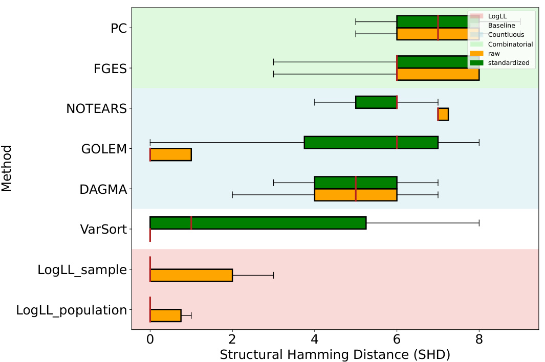
This figure compares the performance of various causal discovery methods on datasets with 5 nodes and 2k expected edges, generated using the Erdős-Rényi (ER) random graph model. The comparison is made between using raw data and standardized data. The results show that the Structural Hamming Distance (SHD), a measure of the difference between the estimated graph and the true graph, is generally lower for methods using raw data, especially for the LOGLL methods (which are the main focus of the paper). This indicates that standardizing the data can negatively impact the performance of some causal discovery methods.
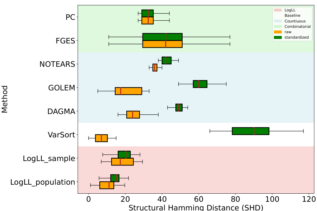
This figure displays the results of an experiment comparing various methods for learning the structure of directed acyclic graphs (DAGs). The experiment uses several types of random graphs with varying numbers of nodes (10, 20, 50, 70, 100) and edges, and evaluates the performance using the Structural Hamming Distance (SHD), a measure of how similar the learned structure is to the true structure. Lower SHD values indicate better performance. The figure is organized with columns representing different graph density levels (k = 1, 2, 4) and rows representing different graph types (Erdős-Rényi and Scale-Free). The number of samples used in each experiment is 1000 (n=1000).
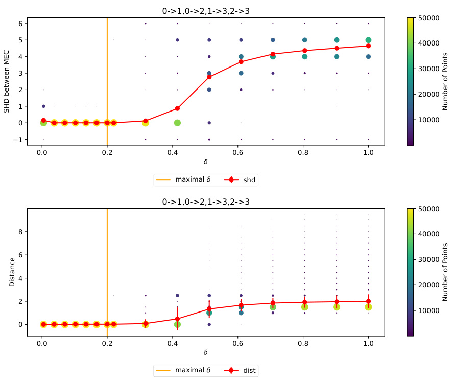
This figure shows the results of an experiment to test the impact of the hyperparameter δ (delta) on the performance of an algorithm for learning causal graphs. The experiment uses a simple fork structure graph (X0 → X1, X0 → X2) as the ground truth graph. The results show that when δ is smaller than a certain threshold (δ0), the algorithm finds the minimal model (Best) within the Markov equivalence class and the structural Hamming distance (SHD) between the estimated graph and the true graph is close to zero. This suggests that choosing δ appropriately leads to accurate causal discovery.
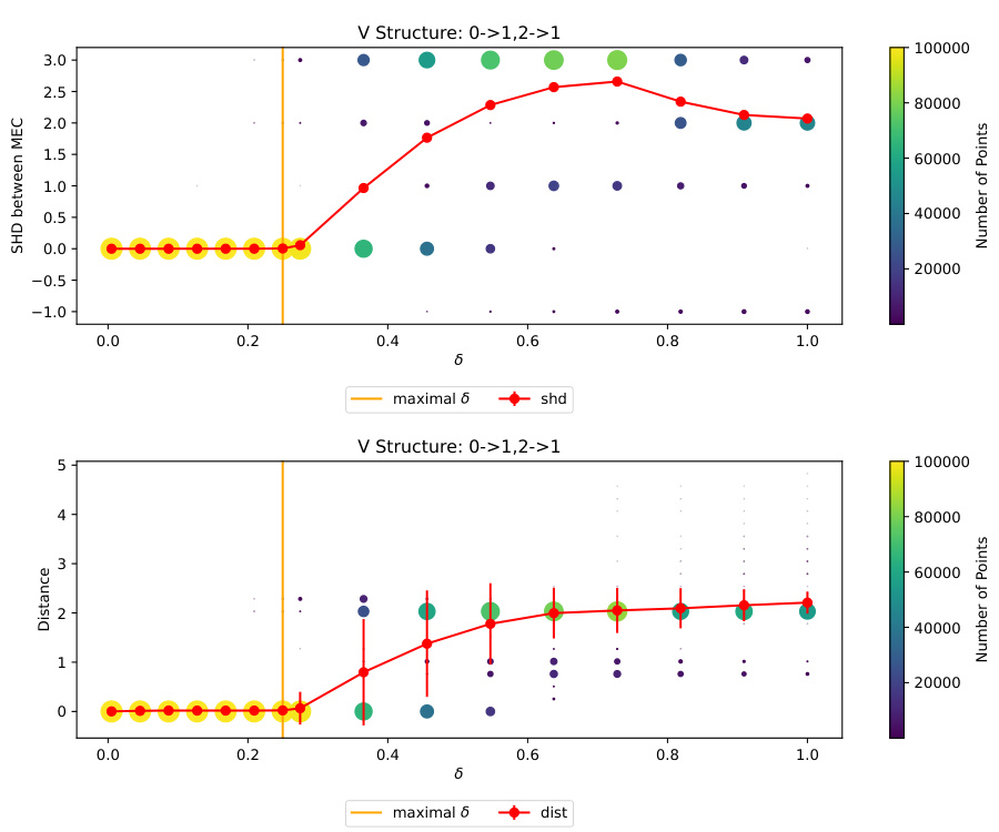
This figure shows the results of an experiment to evaluate the impact of the hyperparameter δ on the performance of a structure learning algorithm. The algorithm aims to recover the minimal equivalence class of a DAG. The X-axis shows the values of δ, while the Y-axes show the structural Hamming distance (SHD) and the distance between the estimated model and the true model. The dots represent the results from 100000 different initializations of the algorithm, showing the distribution of SHD and distance values for each δ value. The red line shows the average values, highlighting that for small enough δ values (0 < δ < δ0), the algorithm consistently recovers the minimal equivalence class.
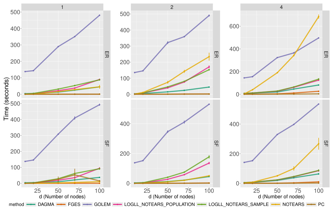
The figure displays the time taken by different causal discovery algorithms to learn the graph structure for various graph sizes (number of nodes) and edge densities. The algorithms are compared using the Structural Hamming Distance (SHD), which measures how close the estimated graph structure is to the ground truth. The graph types considered are Erdős-Rényi (ER) and Scale-Free (SF) networks, characterized by different connectivity patterns. The results show how the computation time increases with the number of nodes and edges. The time taken by our proposed method is comparable to other state-of-the-art methods.
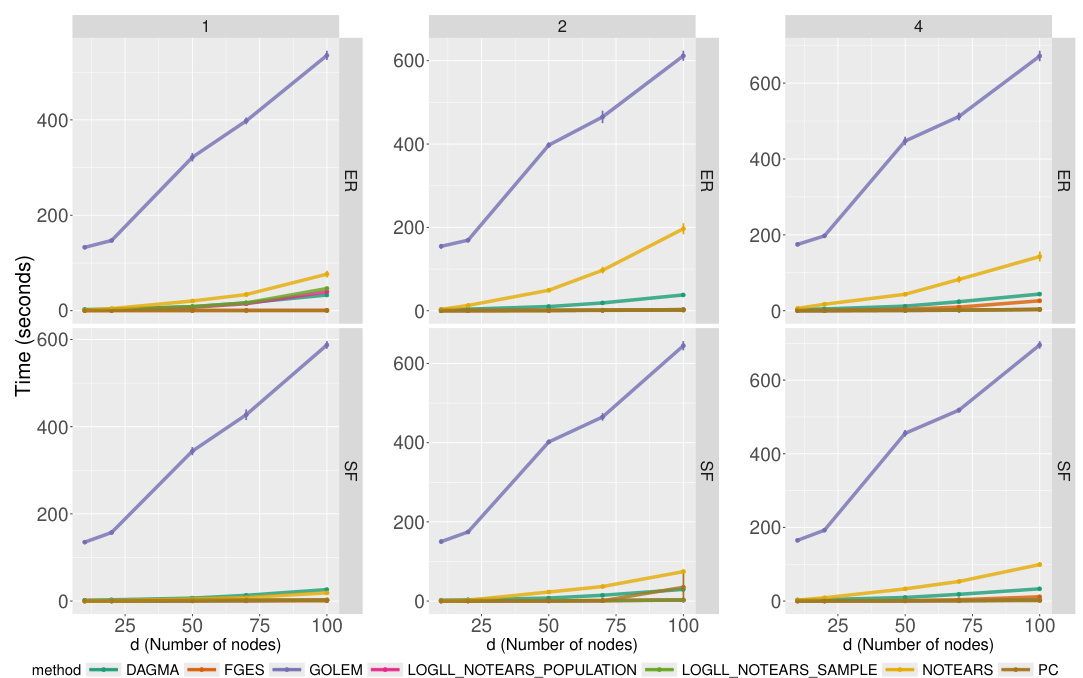
This figure shows the computation time for different causal structure learning algorithms on raw data. The x-axis represents the number of nodes in the graph, and the y-axis shows the time taken (in seconds). Different colors represent different algorithms. The results are broken down by the type of graph (Erdős-Rényi or Scale-free) and the average number of edges. The standard error bars have been removed for clarity.
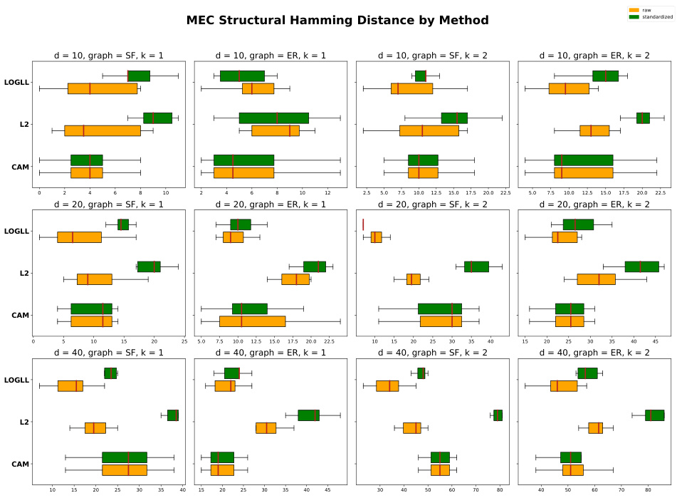
This figure displays the results of the Structural Hamming Distance (SHD) for neural network models with different graph types (scale-free and Erdős-Rényi) and numbers of nodes. The SHD measures the difference between the estimated causal graph structure and the ground truth. Two methods are compared: LOGLL (using log-likelihood with quasi-MCP penalty) and L2 (using least squares loss with L1 penalty), along with a CAM baseline. The results show the impact of standardization on the SHD for both methods, across various network settings and sizes.
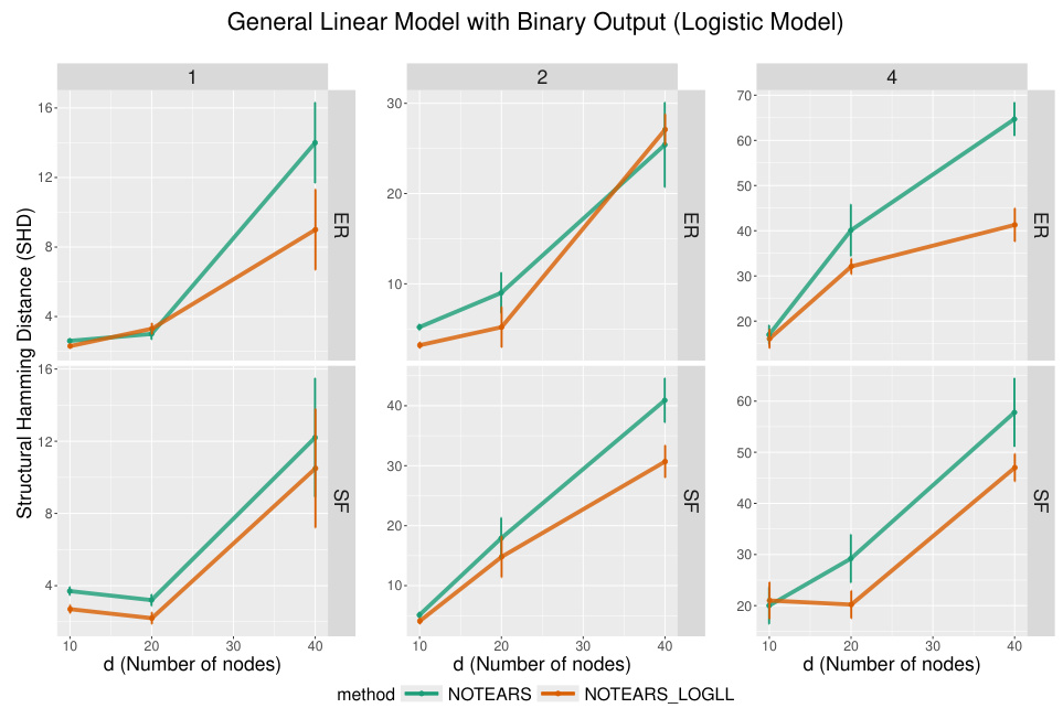
The figure shows the comparison of the SHD for the logistic model between NOTEARS and LOGLL-NOTEARS with different number of nodes. The results are shown for scale-free and Erdos-Renyi graphs with different numbers of expected edges. The error bars show the standard error over 10 simulations.
Full paper#


