TL;DR#
Many online platforms, such as ride-sharing apps and e-commerce marketplaces, rely on dynamic pricing of service fees to maximize revenue. This study tackles the real-world complexity of this task, acknowledging three key challenges: initially unknown buyer demand, the inability to directly observe demand information (only equilibrium prices and quantities are visible), and strategic buyer behavior (customers might manipulate their demand to influence prices). These difficulties make traditional pricing models and estimations unreliable.
This paper proposes novel algorithms to dynamically set service fees. The algorithms incorporate active randomness injection for effective exploration and exploitation, instrumental variable methods for accurate demand estimation using non-i.i.d. actions (service fees), and a low-switching cost design to mitigate strategic buyer behavior. The researchers prove that their approach achieves an optimal regret bound, demonstrating its effectiveness in balancing revenue maximization with learning the unknown demand. The study also reveals the counterintuitive benefit of incorporating randomness in supply to assist with learning.
Key Takeaways#
Why does it matter?#
This paper is crucial for researchers in pricing, revenue management, and algorithmic economics. It provides novel solutions to a practically relevant problem—optimizing service fees on third-party platforms—by introducing a new method that balances exploration and exploitation. It also offers important theoretical guarantees (optimal regret bounds) and insights into the use of actions as instruments, low-switching pricing policies, and the role of supply randomness.
Visual Insights#

🔼 This figure shows two Uber ride receipts with different total prices but the same booking fee. It illustrates that while Uber uses a fixed booking fee in a short time period, it may dynamically adjust prices over a longer period to maximize revenue and adapt to demand.
read the caption
Figure 1: Uber. Above are two Uber rides from the same city in February 2024. The price of the two rides differs by nearly double, yet the booking fee remains at $1.27 for both, suggesting that a fixed booking fee mechanism might be employed in February. However, over a longer period of time, Uber may switch to a dynamic pricing strategy.
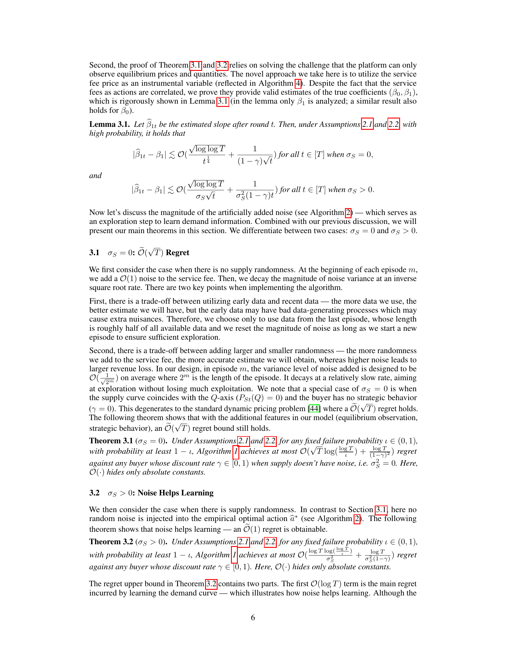
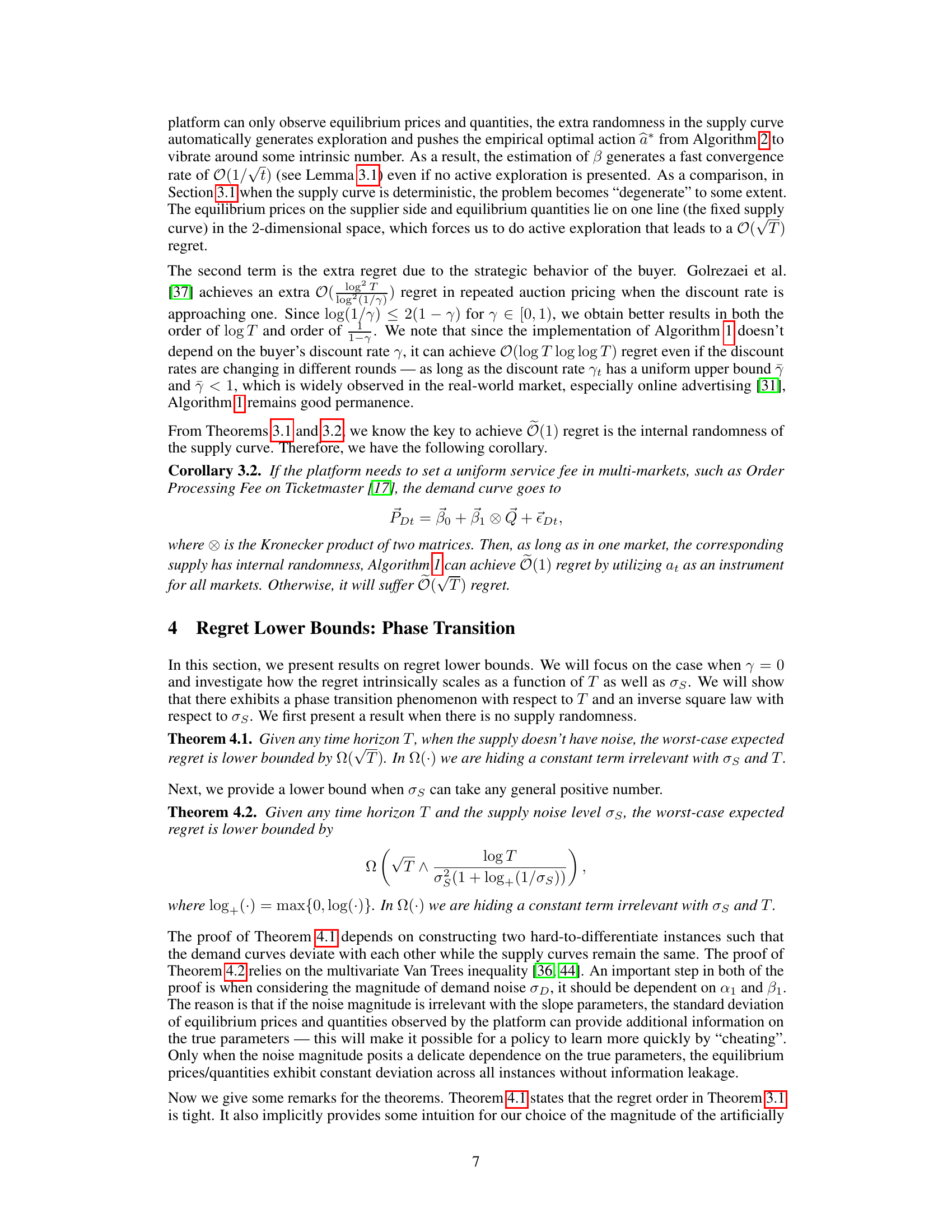
🔼 This figure displays the 95% confidence intervals of the regret obtained by Algorithm 1 over 10 separate trajectories. The left panel shows results when there is supply randomness (σς = 1), while the right panel shows the results when there is no supply randomness (σς = 0). The figure visually represents the performance of the algorithm under different conditions and demonstrates the impact of supply randomness on the regret.
read the caption
Figure 2: 95% confidence region of regret of Algorithm 1 over 10 trajectories: σε = 1 (left) and σε = 0 (right).
In-depth insights#
Strategic Buyer Models#
Strategic buyer models are crucial for accurately representing buyer behavior in dynamic pricing scenarios. Rational buyers, unlike myopic models, consider the platform’s pricing strategy and adjust their purchasing behavior accordingly. This strategic interaction adds significant complexity, as buyers might delay purchases hoping for lower prices, or even misrepresent their preferences to manipulate the platform’s learning process. Modeling this behavior requires considering factors such as discount rates, switching costs, and the information asymmetry between the platform and buyers. Game-theoretic approaches are often employed to capture the strategic element, analyzing equilibrium outcomes and the platform’s optimal pricing policies. This necessitates considering the buyer’s overall utility maximization problem across multiple time periods, making it essential to balance exploration (learning buyer preferences) and exploitation (optimizing revenue). Robust models must also address the potential for biased estimations caused by strategic buyer behavior and incorporate techniques such as instrumental variables to obtain consistent demand estimates. The resulting models, while more complex, provide more accurate predictions of market responses to pricing strategies, ultimately leading to improved revenue management for the platform.
Active Randomness#
Active randomness in the context of dynamic pricing and demand learning presents a powerful strategy to mitigate the exploration-exploitation dilemma. By injecting controlled randomness into pricing decisions, the platform can actively gather information about the demand curve, even when facing strategic buyers who might otherwise try to manipulate the system to their advantage. This approach contrasts with passive observation which relies on simply observing market outcomes. Active randomness allows for a more direct and efficient way to learn about the demand landscape. It’s particularly effective in scenarios where demand information is initially unknown and the system dynamics are influenced by both demand and supply randomness. However, the design and implementation of active randomness require careful consideration. The level of randomness needs to be carefully tuned to balance information gathering (exploration) and revenue maximization (exploitation). Too little randomness results in poor learning, while too much leads to significant revenue loss. Further, the type of randomness (e.g., additive vs. multiplicative) and its effect on buyer behavior must be carefully considered. Overall, active randomness represents a sophisticated strategy that leverages controlled uncertainty to improve the efficiency of demand learning and ultimately, optimize revenue generation in complex, dynamic pricing environments.
IV Demand Estimation#
Instrumental variable (IV) techniques offer a powerful approach to demand estimation in settings where traditional methods are hampered by endogeneity. The core idea is to use an instrumental variable (Z) that is correlated with the treatment variable (price) but uncorrelated with the error term in the demand model, thus addressing omitted variable bias and simultaneity. In the context of dynamic service fee pricing, actions (fee choices) can be employed as instruments, leveraging their predictable influence on transaction quantities. However, the non-independence of actions over time presents a significant challenge. The paper’s innovation lies in showing how, despite this correlation, carefully designed actions can still provide consistent estimates. The use of IV methods, particularly with non-i.i.d. instruments, offers a significant contribution to the field of online pricing and demand learning, highlighting how clever experimentation can extract valuable information from seemingly noisy data. The authors cleverly use the fact that the platform sets the fee before the buyer responds, thus establishing a causal link between actions and outcomes. Importantly, their approach incorporates the strategic behavior of buyers, a critical factor often ignored, and quantifies the effects of supply randomness on estimation accuracy. This is not just a technical contribution but also improves our understanding of price optimization under realistic market dynamics.
Low-Switching Cost#
The concept of “Low-Switching Cost” in dynamic pricing strategies, particularly within the context of third-party platforms and strategic buyers, offers valuable insights. Low switching costs encourage buyers to act in a more truthful manner, reducing the incentive for strategic misrepresentation of preferences to manipulate future prices. By minimizing the penalty for frequent changes, the platform can more effectively explore the demand landscape while mitigating the risks associated with buyers who might intentionally withhold demand information to influence future prices. This approach allows the algorithm to balance exploration and exploitation better, leading to improved revenue generation in the long run. However, the effectiveness of low-switching costs is intrinsically linked to buyer patience and the time horizon of the pricing strategy. If buyers are extremely patient, the benefits of low-switching costs may be diminished, and alternative mechanisms may be needed to encourage truthful buyer behavior. The optimal switching cost is a function of buyer patience and supply randomness, highlighting the importance of considering the specific market characteristics when implementing this strategy.
Phase Transition#
The concept of ‘Phase Transition’ in the context of dynamic pricing models, as discussed in the research paper, is a crucial finding that reveals a fundamental shift in the system’s behavior. The existence of a phase transition point signifies that the system’s performance, specifically the regret, drastically changes as a parameter crosses a critical threshold. In this specific scenario, the level of randomness in the supply (σs) acts as the critical parameter. Below the threshold, the regret scales suboptimally with the time horizon (T). However, once the supply randomness surpasses the threshold, the regret transitions to a substantially lower, and arguably more desirable, level; it approaches optimality. This transition highlights the importance of supply randomness in the learning process. It suggests that introducing controlled randomness in the supply can greatly enhance the platform’s ability to efficiently learn the demand curve and optimize revenue. This is an intriguing counter-intuitive result, as randomness is often associated with suboptimal performance. However, this model demonstrates how strategic injection of randomness can facilitate a phase transition to a regime of much improved efficiency, offering valuable insights for designing dynamic pricing strategies in real-world settings.
More visual insights#
More on figures
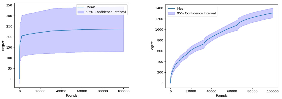
🔼 This figure displays the 95% confidence intervals for the regret of Algorithm 1 across 10 separate simulation runs. The left panel shows results when there is randomness in the supply (σs = 1), while the right panel shows results in the absence of supply randomness (σs = 0). The y-axis represents the cumulative regret, and the x-axis represents the number of rounds (time). The figure visually demonstrates the impact of supply randomness on the algorithm’s performance and regret.
read the caption
Figure 2: 95% confidence region of regret of Algorithm 1 over 10 trajectories: σs = 1 (left) and σs = 0 (right).

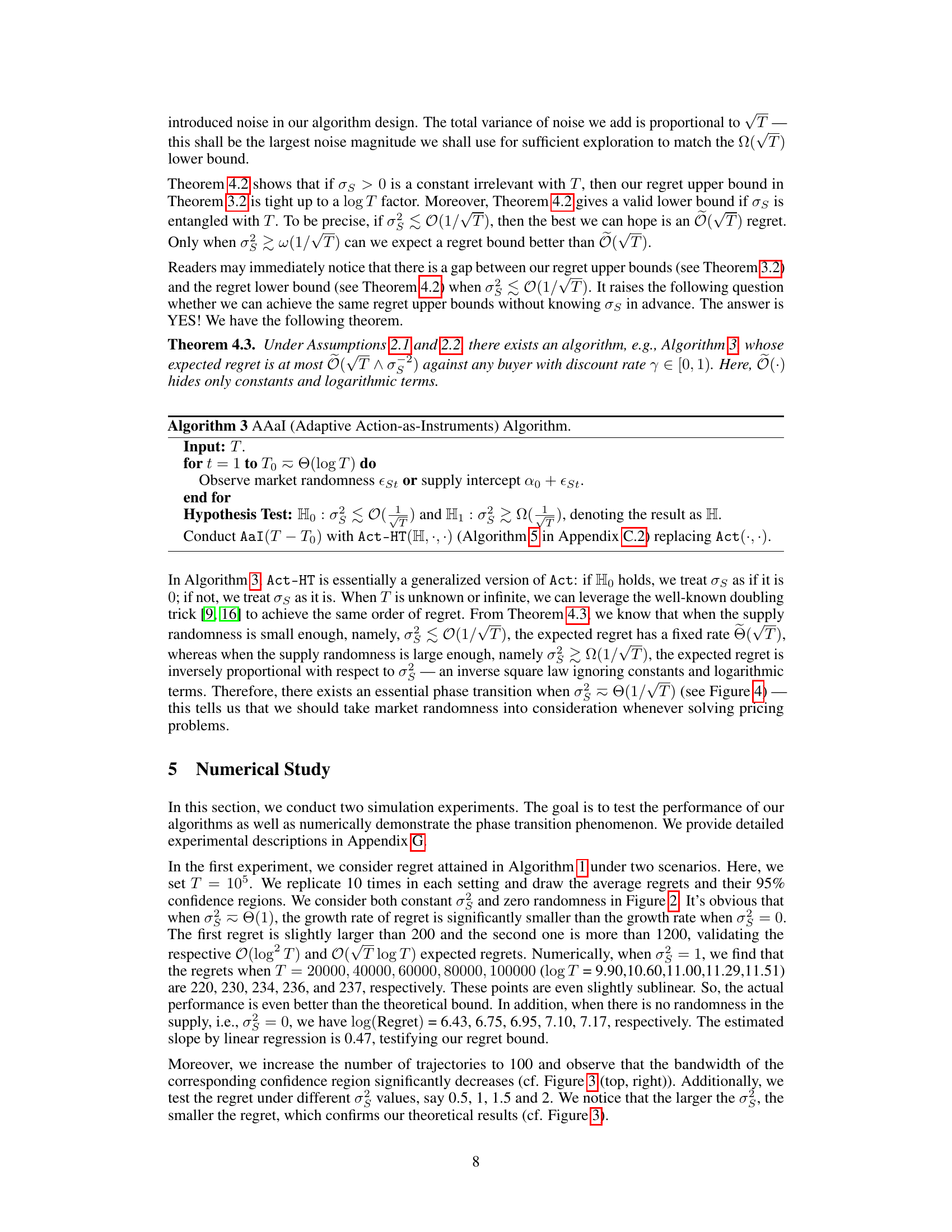
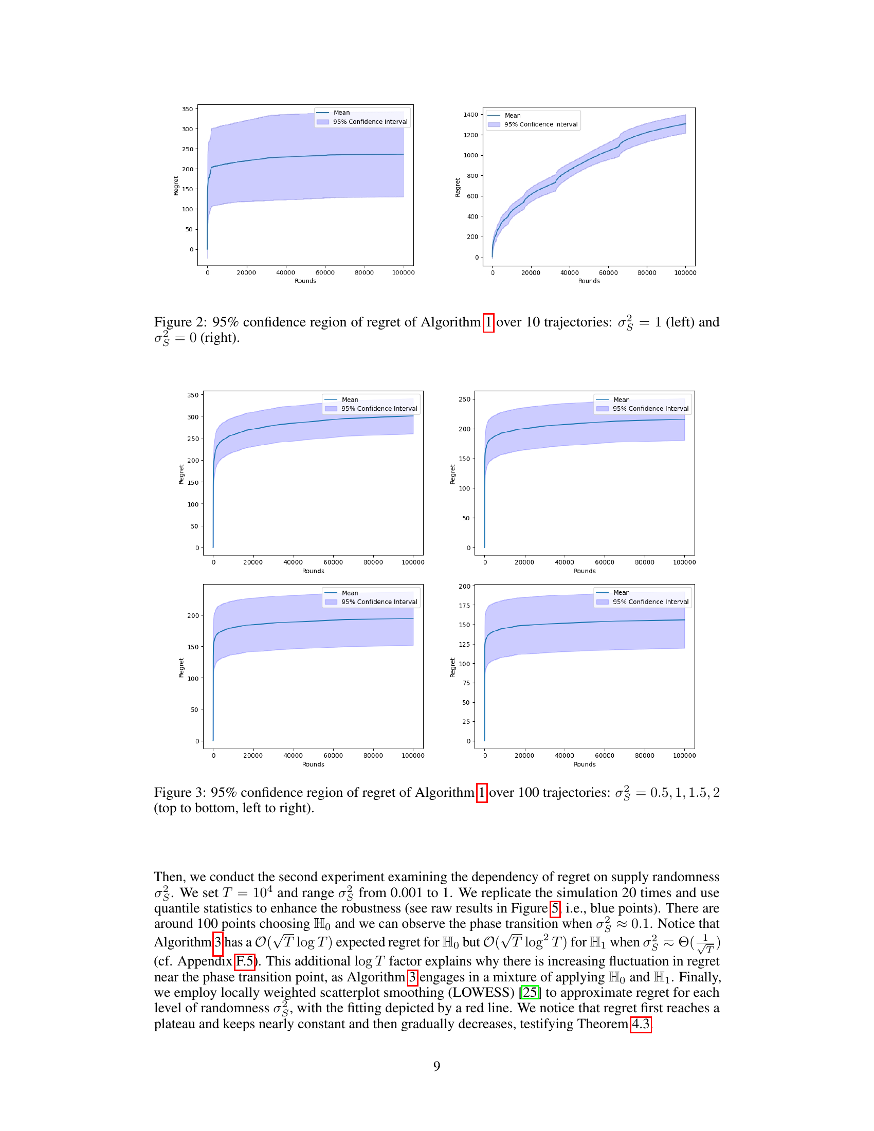
🔼 This figure shows the 95% confidence region of the regret of Algorithm 1 across 100 simulation trajectories. Four scenarios are presented, each with a different level of supply randomness (σs): 0.5, 1, 1.5, and 2. The plots illustrate the impact of varying supply randomness on the algorithm’s performance, showing how regret changes over time (rounds). The confidence intervals give a sense of the variability of the results across the multiple simulation runs.
read the caption
Figure 3: 95% confidence region of regret of Algorithm 1 over 100 trajectories: σε = 0.5, 1, 1.5, 2 (top to bottom, left to right).
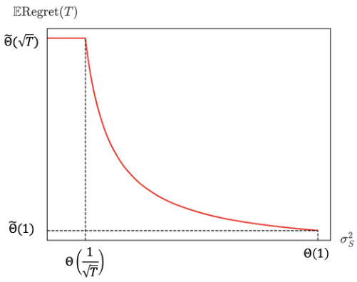
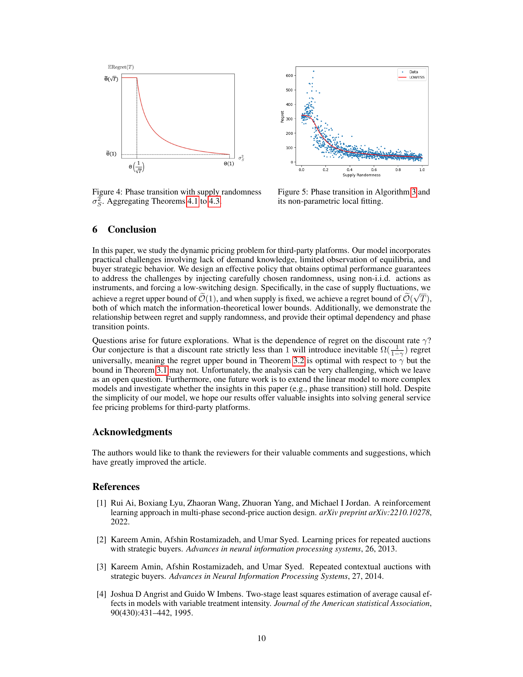
🔼 This figure shows the phase transition phenomenon of the regret with respect to supply randomness (σs). When the supply randomness is low (σs ≤ O(1/√T)), the regret scales as O(√T). However, when the supply randomness is high (σs ≥ Ω(1/√T)), the regret decreases significantly to O(1). The figure visually represents the theoretical results from Theorems 4.1, 4.2, and 4.3, demonstrating how the introduction of randomness in supply affects the learning process and the overall regret.
read the caption
Figure 4: Phase transition with supply randomness σs. Aggregating Theorems 4.1 to 4.3.
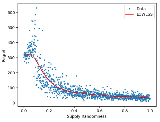
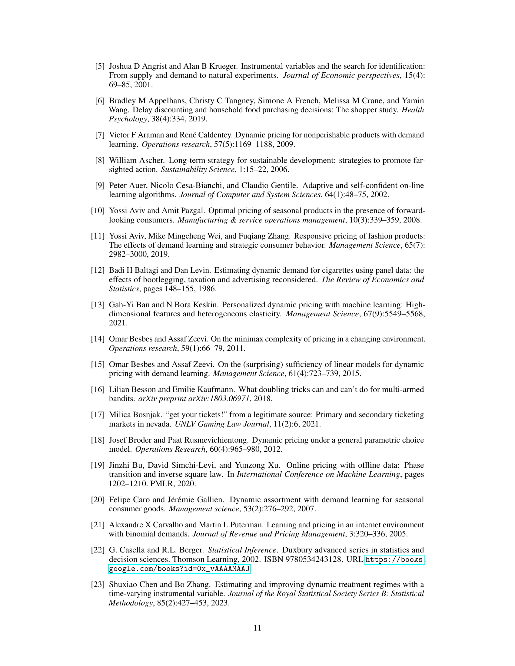
🔼 This figure shows the results of the second numerical experiment, where the regret is plotted against different levels of supply randomness (σs). The blue dots represent the raw data, and the red line shows the results of locally weighted scatterplot smoothing (LOWESS). The plot shows a clear phase transition around σs ≈ 0.1, where the regret decreases significantly as supply randomness increases. This is consistent with the theoretical findings of the paper, indicating that supply randomness can significantly help with the learning of demand information.
read the caption
Figure 5: Phase transition in Algorithm 3 and its non-parametric local fitting.
More on tables

🔼 This algorithm calculates the optimal service fee by maximizing the expected revenue, considering the supply and demand curves. It then adds a noise term to the optimal fee to facilitate exploration, specifically when there’s no randomness in the supply. The noise’s variance decreases over time. The output is the final service fee.
read the caption
Algorithm 2 Act Algorithm.

🔼 This algorithm takes datasets D and A as input and performs an instrumental variable regression to estimate the parameters β0 and β1 of the demand curve. It first regresses equilibrium quantity Qe and price Pe on the service fee at, obtaining estimates â0, â1, ˆb0, ˆb1. Then it calculates the sample means of Qe and Pe, denoted by Qe and Pe, and estimates β1 as the ratio of ˆb1 to ˆa1. Finally, it estimates β0 using the sample mean Pe, estimated β1, and sample mean Qe. The output is (βˆ0, βˆ1), the estimated parameters of the demand curve.
read the caption
Algorithm 4 IV Algorithm.

🔼 This figure presents the results of simulation experiments conducted to evaluate the performance of Algorithm 1 under different levels of supply randomness (σs). The plots show the 95% confidence intervals for the regret (difference between the actual revenue and the optimal revenue) across 100 simulation runs for four different values of σs (0.5, 1, 1.5, and 2). The x-axis represents the number of rounds, and the y-axis represents the regret. The results illustrate how the regret changes with different amounts of supply randomness.
read the caption
Figure 3: 95% confidence region of regret of Algorithm 1 over 100 trajectories: σs = 0.5, 1, 1.5, 2 (top to bottom, left to right).

🔼 This figure displays the 95% confidence intervals for the regret of Algorithm 1 across 10 separate simulation runs. The left panel shows results when there is supply randomness (σs = 1), while the right panel shows results when there is no supply randomness (σs = 0). The results illustrate the impact of supply randomness on the algorithm’s performance and regret.
read the caption
Figure 2: 95% confidence region of regret of Algorithm 1 over 10 trajectories: σs = 1 (left) and σs = 0 (right).
Full paper#

