TL;DR#
Current methods for improving classifier robustness often rely on expensive synthetic data generation or complex augmentation strategies. This can be problematic, especially in data-scarce environments. The existing augmentation techniques also often fail to adequately address several crucial robustness challenges, such as out-of-distribution detection and certified adversarial accuracy.
This paper introduces DiffAug, a novel augmentation technique that leverages diffusion models. DiffAug is computationally efficient, requiring only a single forward and reverse diffusion step, making it suitable for large datasets and resource-constrained environments. Importantly, DiffAug does not require any additional data. The research demonstrates its effectiveness across various robustness benchmarks, including improvements in covariate shift robustness, certified adversarial accuracy, and out-of-distribution detection. The findings also suggest a connection between perceptually aligned gradients and robustness.
Key Takeaways#
Why does it matter?#
This paper is crucial for researchers seeking to improve classifier robustness. It introduces a novel, computationally efficient augmentation technique, DiffAug, that doesn’t require additional data, addressing a key limitation in current methods. DiffAug’s effectiveness across various robustness benchmarks, combined with its compatibility with existing techniques, makes it a valuable tool. The paper’s exploration of perceptual gradient alignment offers new avenues for understanding and improving classifier training. This opens up several new research opportunities.
Visual Insights#
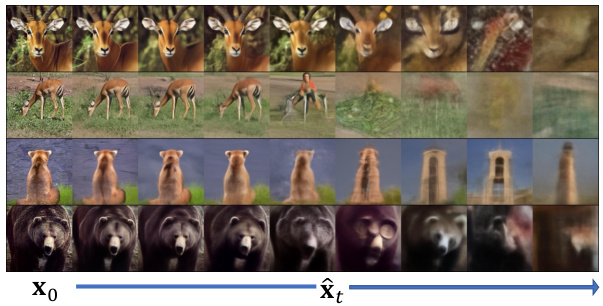
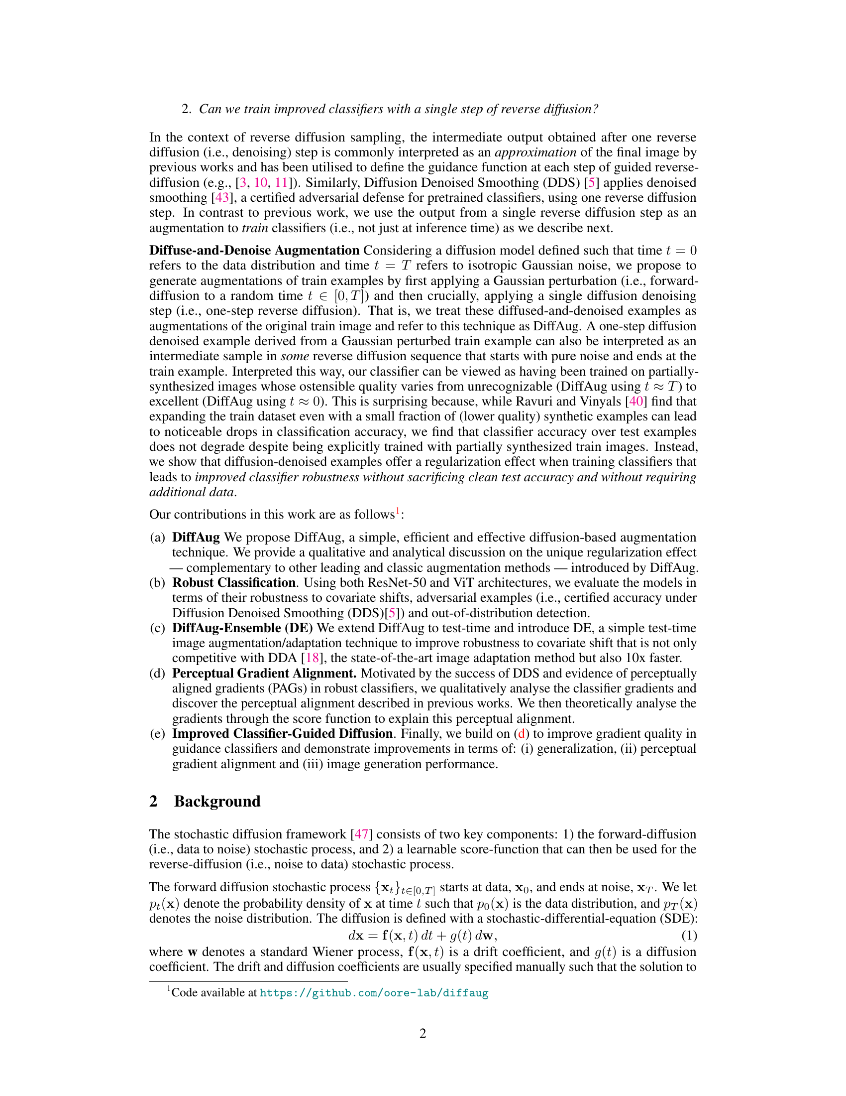
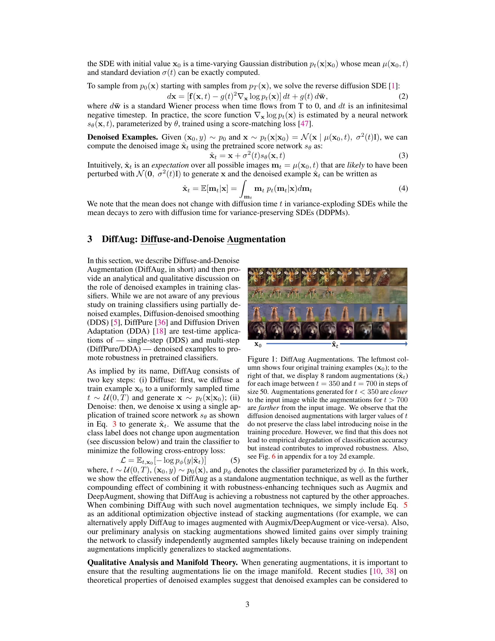
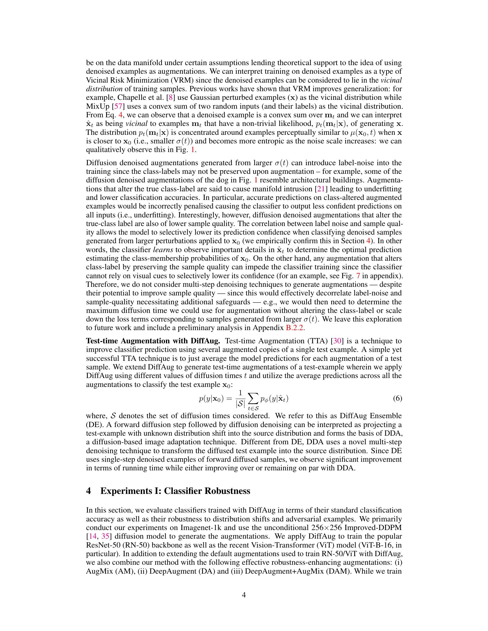
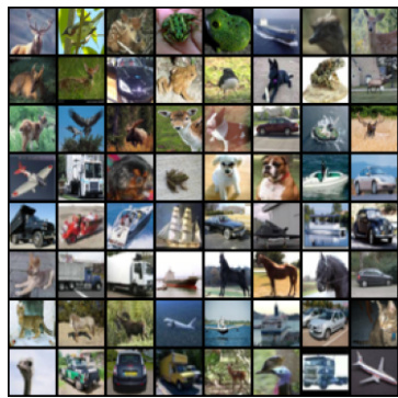
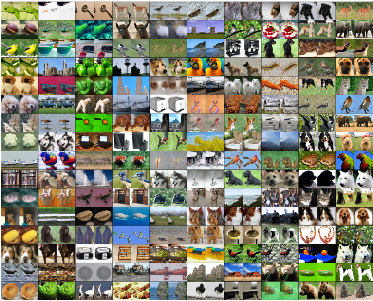
🔼 This figure shows examples of augmentations generated using the DiffAug method. Four original images are shown in the leftmost column, followed by eight augmented versions of each image generated using different diffusion times (t). The augmentations demonstrate how the forward and reverse diffusion steps transform the original images, with augmentations generated at smaller t values being more similar to the original images than those at larger t values. The figure illustrates that DiffAug introduces noise into the training process, by sometimes altering the class label of the image. However, it also shows that this doesn’t negatively impact the classification accuracy of the model, and in fact contributes to its robustness.
read the caption
Figure 1: DiffAug Augmentations. The leftmost column shows four original training examples (x0); to the right of that, we display 8 random augmentations (xt) for each image between t = 350 and t = 700 in steps of size 50. Augmentations generated for t < 350 are closer to the input image while the augmentations for t > 700 are farther from the input image. We observe that the diffusion denoised augmentations with larger values of t do not preserve the class label introducing noise in the training procedure. However, we find that this does not lead to empirical degradation of classification accuracy but instead contributes to improved robustness. Also, see Fig. 6 in appendix for a toy 2d example.

🔼 This table presents the top-1 accuracy results on ImageNet-C (with severity level 5) and ImageNet-Test datasets. It shows the performance of different classifier models trained with various augmentation techniques. The augmentation techniques include AugMix (AM), DeepAugment (DA), AugMix+DeepAugment (DAM), and the proposed DiffAug method, either alone or in combination with the others. The evaluation is done using four modes: DDA (Diffusion-based test-time adaptation), DDA+Self-Ensemble (DDA+SE), DiffAug Ensemble (DE), and Default (without test-time augmentation). The average accuracy across all corruption types and evaluation modes is presented.
read the caption
Table 1: Top-1 Accuracy (%) on Imagenet-C (severity=5) and Imagenet-Test. We summarize the results for each combination of Train-augmentations and evaluation modes. The average (avg) accuracies for each classifier and evaluation mode is shown.
In-depth insights#
DiffAug: Robustness Boost#
The concept of “DiffAug: Robustness Boost” proposes a novel data augmentation technique to enhance the robustness of image classifiers. DiffAug leverages diffusion models, a powerful class of generative models, performing a single forward and reverse diffusion step on each training image. This process subtly alters the image while maintaining its class label, creating a form of regularized augmentation that improves classifier performance on various benchmarks. The method is particularly effective in improving robustness to covariate shift, adversarial examples, and out-of-distribution detection. The simplicity and computational efficiency of DiffAug are highlighted as key advantages, and its compatibility with other augmentation techniques is explored, further demonstrating its versatility. Combining DiffAug with existing methods often leads to synergistic improvements in robustness, making it a valuable tool for training robust and reliable classifiers. The unique regularization effect offered by DiffAug complements existing techniques and contributes to a more robust and generalized classifier.
Single-Step Diffusion#
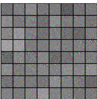
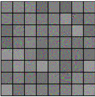
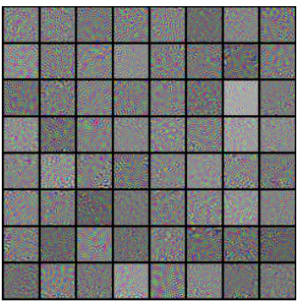
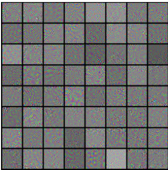
The concept of “Single-Step Diffusion” in the context of diffusion models for image generation and classification presents a compelling trade-off between computational efficiency and model performance. Traditional diffusion models require numerous iterative steps for effective denoising, leading to high computational costs. A single-step approach drastically reduces this burden, making it more practical for applications with limited resources. The key challenge lies in maintaining sufficient sample quality with only a single denoising step. This might necessitate more sophisticated denoising networks or careful selection of hyperparameters. While the quality of single-step diffusion might be lower than multi-step, its efficiency gains could be significant, particularly in scenarios like real-time augmentation or applications with strict latency constraints. The efficacy of single-step diffusion would heavily depend on the specific diffusion model architecture and the data it was trained on. Further research should investigate whether single-step diffusion can be successfully applied to different model architectures, datasets, and downstream tasks (e.g., image classification, anomaly detection). The impact on robustness and generalization capabilities also warrants detailed exploration. It is crucial to analyze the balance between computational efficiency and performance degradation compared to multi-step approaches.
PAGs & Generalization#
The concept of Perceptually Aligned Gradients (PAGs) and their connection to generalization in machine learning models is a fascinating area of research. PAGs refer to gradients that align with human perception of visual features, making them intuitively meaningful and interpretable. The hypothesis is that models exhibiting PAGs are better at generalizing because their learning process is more aligned with how humans understand visual information. This is particularly relevant to image classification tasks, where the ability to discern subtle visual differences is crucial for accurate and robust classification across diverse datasets. A key question is whether the presence of PAGs is a cause or effect of improved generalization. There may be other factors underlying good generalization, such as model architecture or regularization techniques, and it’s essential to decouple these effects to truly understand the role of PAGs. Further investigation could explore whether techniques explicitly designed to promote PAGs lead to demonstrably better generalization performance, or if improved generalization naturally fosters the emergence of PAGs during the learning process. The relationship between gradient alignment and generalization remains an active research topic, with potential to significantly improve model performance and interpretability.
CG Diffusion Enhance#
In the context of classifier-guided diffusion, the enhancement strategies focus on improving the quality and alignment of classifier gradients. A suboptimal guidance signal can hinder the generation of high-fidelity images. By leveraging techniques such as denoising augmentation, the goal is to refine the guidance signal and ensure that the classifier directs the diffusion process towards perceptually meaningful variations. Improved gradient alignment leads to more coherent and realistic image synthesis. Moreover, the efficiency of the guidance process is important; therefore, enhancing CG diffusion may involve optimizing the computational cost by employing efficient sampling techniques and architectures. This could involve incorporating techniques from other generative modeling methods or developing novel algorithms designed to reduce the number of steps involved in the diffusion process while preserving the quality of the results. Ultimately, enhancing classifier-guided diffusion aims at generating high-quality, diverse, class-conditional samples by improving gradient quality, computational efficiency, and overall model performance.
Future Work: DiffAug#
Future research directions for DiffAug could explore several promising avenues. Extending DiffAug to other generative models beyond diffusion models, such as GANs or VAEs, could broaden its applicability and potentially reveal new regularization effects. Investigating the theoretical underpinnings of DiffAug’s regularization properties through a deeper analysis of the diffusion process and its interaction with classifier training is crucial. Combining DiffAug with other augmentation techniques in more sophisticated ways, going beyond simple concatenation, might unlock synergistic benefits. Exploring DiffAug’s effectiveness across a wider range of tasks and datasets, including those beyond image classification, could also provide valuable insights. Finally, a comprehensive study evaluating the impact of various diffusion model architectures and training strategies on DiffAug’s performance would further solidify its potential.
More visual insights#
More on figures

🔼 The figure shows the average prediction entropy of different models trained with and without DiffAug on Imagenet test data, plotted against different diffusion times. The models trained with DiffAug show higher entropy (lower confidence) at larger diffusion times, which correspond to images with more noise or imperceptible details. This indicates that DiffAug helps the model to be more uncertain about noisy or unclear images, a desirable trait for robust classification. The unexpected finding that models without DiffAug do not assign random labels to highly-noisy images is also highlighted.
read the caption
Figure 2: Average prediction entropy on DiffAug samples vs diffusion time measured with Imagenet-Test. We observe that the models trained with DiffAug correctly yield predictions with higher entropies (lower confidence) for images containing imperceptible details (i.e. larger t). Surprisingly, the classifiers trained without DiffAug do not also assign random-uniform label distribution for DiffAug images at t = 999, which have no class-information by construction. Also, see Fig. 11.
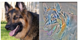
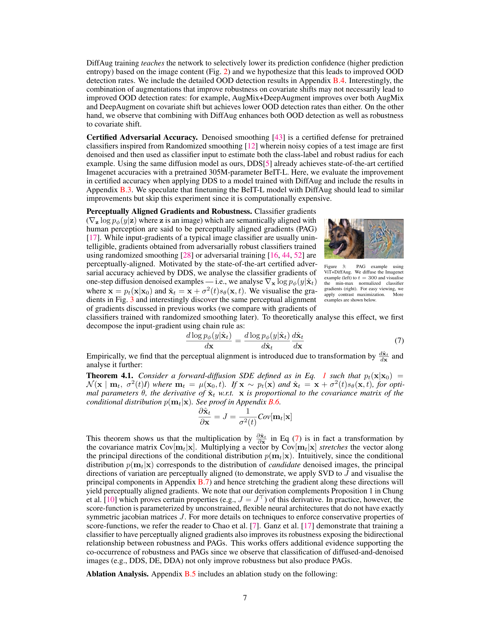
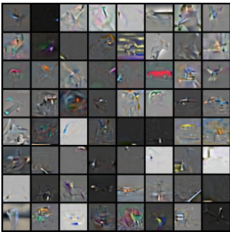
🔼 This figure shows an example of perceptually aligned gradients (PAGs) obtained by using the DiffAug method with Vision Transformer (ViT) architecture. The left panel shows the original Imagenet image. The image is diffused to time t = 300 using the forward diffusion process, and then the min-max normalized classifier gradients are visualized in the right panel. Contrast maximization is applied to enhance the visibility of the gradients. The gradients appear perceptually aligned with the image content, indicating that the classifier is learning meaningful features that are aligned with human perception.
read the caption
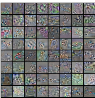
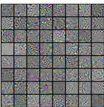
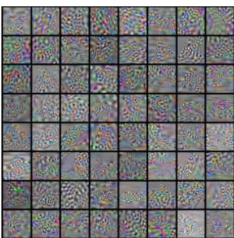
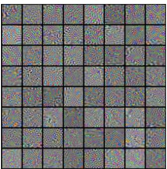
Figure 3: PAG example using ViT+DiffAug. We diffuse the Imagenet example (left) to t = 300 and visualise the min-max normalized classifier gradients (right). For easy viewing, we apply contrast maximization. More examples are shown below.

🔼 This figure shows the effect of DiffAug on four example images. The leftmost column shows the original images. The remaining columns show the results of applying DiffAug with different diffusion times (t). As t increases, the augmentation becomes more distinct from the original image. Interestingly, even when the augmentations significantly alter the image and sometimes change the class label, the model’s accuracy does not suffer, but rather improves robustness.
read the caption
Figure 1: DiffAug Augmentations. The leftmost column shows four original training examples (x0); to the right of that, we display 8 random augmentations (xt) for each image between t = 350 and t = 700 in steps of size 50. Augmentations generated for t < 350 are closer to the input image while the augmentations for t > 700 are farther from the input image. We observe that the diffusion denoised augmentations with larger values of t do not preserve the class label introducing noise in the training procedure. However, we find that this does not lead to empirical degradation of classification accuracy but instead contributes to improved robustness. Also, see Fig. 6 in appendix for a toy 2d example.
🔼 This figure shows the effect of DiffAug on four example images. The leftmost column shows the original images. The other columns show augmentations created by DiffAug at different timesteps (t). As t increases, the augmentations become more noisy and less visually similar to the original image. Interestingly, even though some high-t augmentations appear to change the class label of the original image, this does not seem to hurt the classifier’s performance, it seems to increase robustness.
read the caption
Figure 1: DiffAug Augmentations. The leftmost column shows four original training examples (x0); to the right of that, we display 8 random augmentations (xt) for each image between t = 350 and t = 700 in steps of size 50. Augmentations generated for t < 350 are closer to the input image while the augmentations for t > 700 are farther from the input image. We observe that the diffusion denoised augmentations with larger values of t do not preserve the class label introducing noise in the training procedure. However, we find that this does not lead to empirical degradation of classification accuracy but instead contributes to improved robustness. Also, see Fig. 6 in appendix for a toy 2d example.
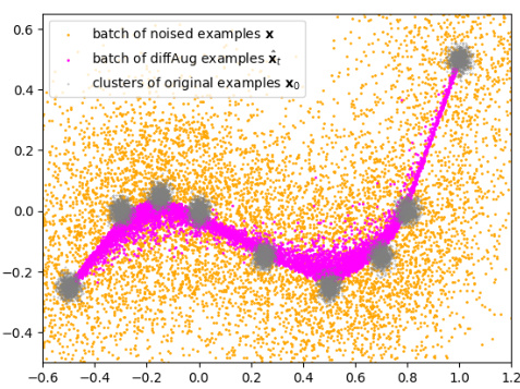
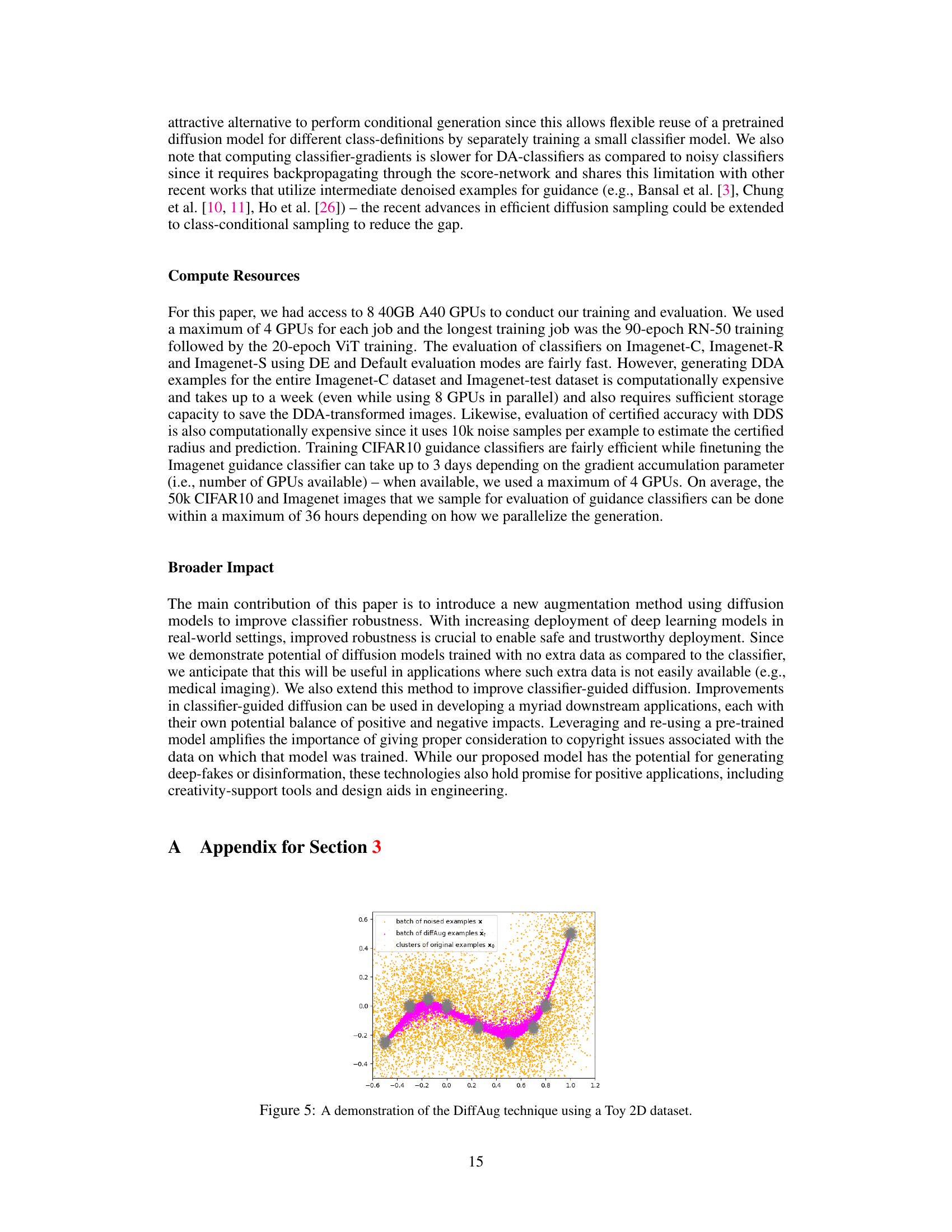
🔼 This figure shows a 2D visualization of the DiffAug process. The orange dots represent the original data points clustered together. The grey dots represent noised examples, dispersed more widely. The magenta line connects a sequence of points illustrating a single example’s journey through the forward and reverse diffusion steps of DiffAug. The final magenta point is the denoised sample after one step of reverse diffusion. This illustrates how DiffAug generates augmented samples that are closer to the data manifold and preserve cluster properties.
read the caption
Figure 5: A demonstration of the DiffAug technique using a Toy 2D dataset.

🔼 This figure shows a 2D visualization of the DiffAug augmentation technique. It illustrates how a training example (black point) is perturbed by the forward diffusion process (red arrows). The reverse diffusion step (green arrows) partially reverses this perturbation, resulting in a set of DiffAug augmented examples (light green points). The figure helps to visualize how DiffAug generates augmentations by combining forward and reverse diffusion steps and that these augmented samples lie on the data manifold.
read the caption
Figure 5: A demonstration of the DiffAug technique using a Toy 2D dataset.

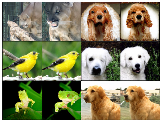
🔼 This figure shows an example of manifold intrusion caused by color augmentation. Hendrycks et al. demonstrate that standard color augmentation can lead to manifold intrusion, where the augmented image is visually different from the original, and the model struggles to use the augmented image for robust classification. The authors contrast this with their proposed DiffAug method, which, while it may change labels, the visual differences between the original and augmented images allow the model to learn from these noisy labels, demonstrating its robustness.
read the caption
Figure 7: Example of Manifold Intrusion from Appendix C of Hendrycks et al. [24]. While DiffAug may alter class labels (Fig. 1), the denoised images are visually distinguishable from the original images allowing the model to also learn from noisy labels without inducing manifold intrusion. On the other hand, here is an example of manifold intrusion where the augmented image does not contain any visual cues that enable the model to be robust to noisy labels.
🔼 This figure shows examples of augmentations generated by DiffAug for four different images. It illustrates how DiffAug diffuses an image to a certain noise level (represented by the time parameter t) and then applies a single step of reverse diffusion, generating a denoised augmented image. The figure shows that with higher values of t, the augmented image is further from the original and can even lose its original class label. However, this noise injection does not negatively affect the final classifier accuracy, and rather it improves its robustness.
read the caption
Figure 1: DiffAug Augmentations. The leftmost column shows four original training examples (x0); to the right of that, we display 8 random augmentations (xt) for each image between t = 350 and t = 700 in steps of size 50. Augmentations generated for t < 350 are closer to the input image while the augmentations for t > 700 are farther from the input image. We observe that the diffusion denoised augmentations with larger values of t do not preserve the class label introducing noise in the training procedure. However, we find that this does not lead to empirical degradation of classification accuracy but instead contributes to improved robustness. Also, see Fig. 6 in appendix for a toy 2d example.
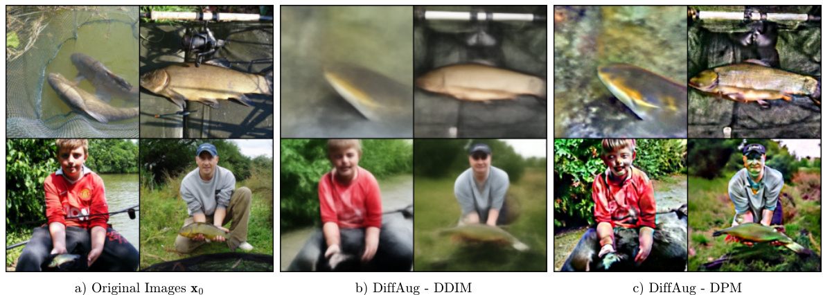
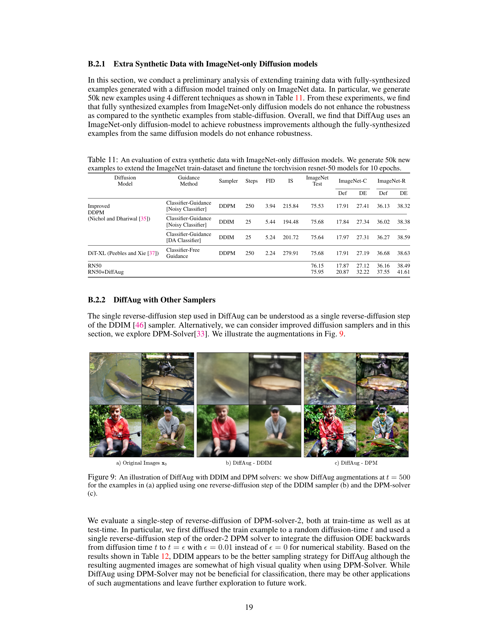
🔼 This figure shows a comparison of different samplers used in the DiffAug method. It illustrates how using different reverse diffusion steps (DDIM and DPM) impacts the final augmentation results. The images show augmentations generated at time step t=500, showing how each sampler handles the process differently.
read the caption
Figure 9: An illustration of DiffAug with DDIM and DPM solvers: we show DiffAug augmentations at t = 500 for the examples in (a) applied using one reverse-diffusion step of the DDIM sampler (b) and the DPM-solver (c).

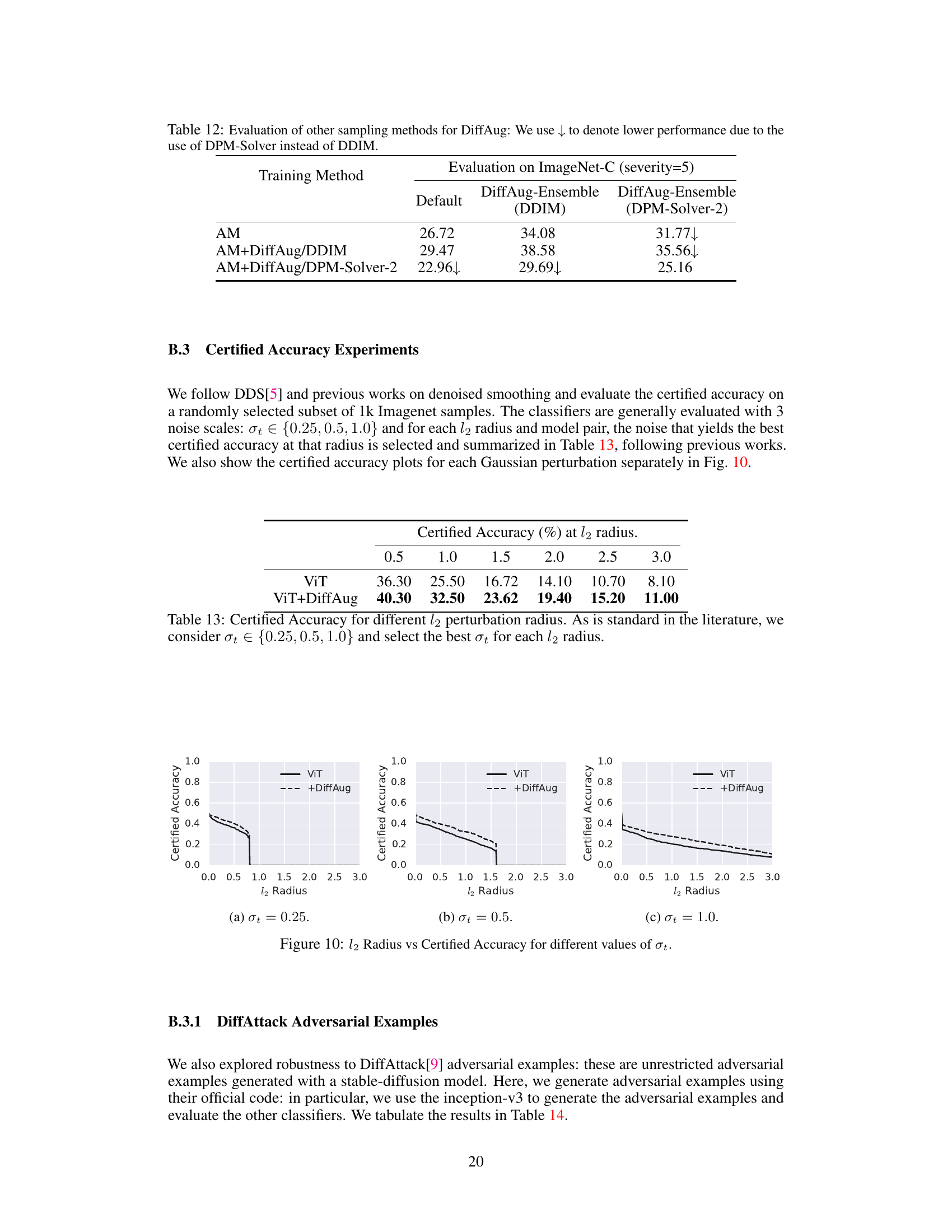
🔼 This figure shows three plots visualizing the relationship between the ℓ2 radius and certified accuracy for different values of the noise scale στ (0.25, 0.5, and 1.0). Each plot compares the performance of a standard ViT model and a ViT model trained with DiffAug. The plots illustrate how the certified accuracy decreases as the ℓ2 radius increases, indicating the robustness of the models against adversarial attacks. The DiffAug-trained model consistently shows higher certified accuracy across all radius values and noise scales, demonstrating the effectiveness of DiffAug in improving the certified robustness of classifiers.
read the caption
Figure 10: ℓ2 Radius vs Certified Accuracy for different values of στ.
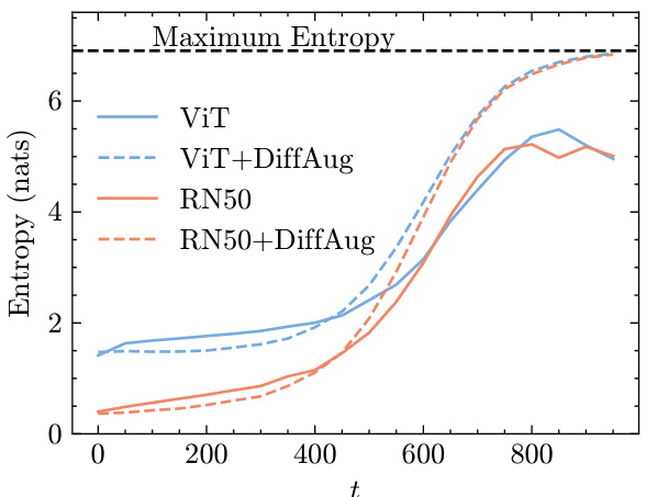
🔼 The figure shows the average prediction entropy of different models (ViT, ViT with DiffAug, ResNet50, ResNet50 with DiffAug) on Imagenet test dataset. The x-axis is the diffusion time (t), and y-axis is the entropy (nats). The figure demonstrates that models trained with DiffAug exhibit higher entropy (lower confidence) for images with more noise (larger t), indicating better out-of-distribution detection capability. Surprisingly, models trained without DiffAug don’t show random uniform label distribution for images with maximum noise (t=999).
read the caption
Figure 2: Average prediction entropy on DiffAug samples vs diffusion time measured with Imagenet-Test. We observe that the models trained with DiffAug correctly yield predictions with higher entropies (lower confidence) for images containing imperceptible details (i.e. larger t). Surprisingly, the classifiers trained without DiffAug do not also assign random-uniform label distribution for DiffAug images at t = 999, which have no class-information by construction. Also, see Fig. 11.

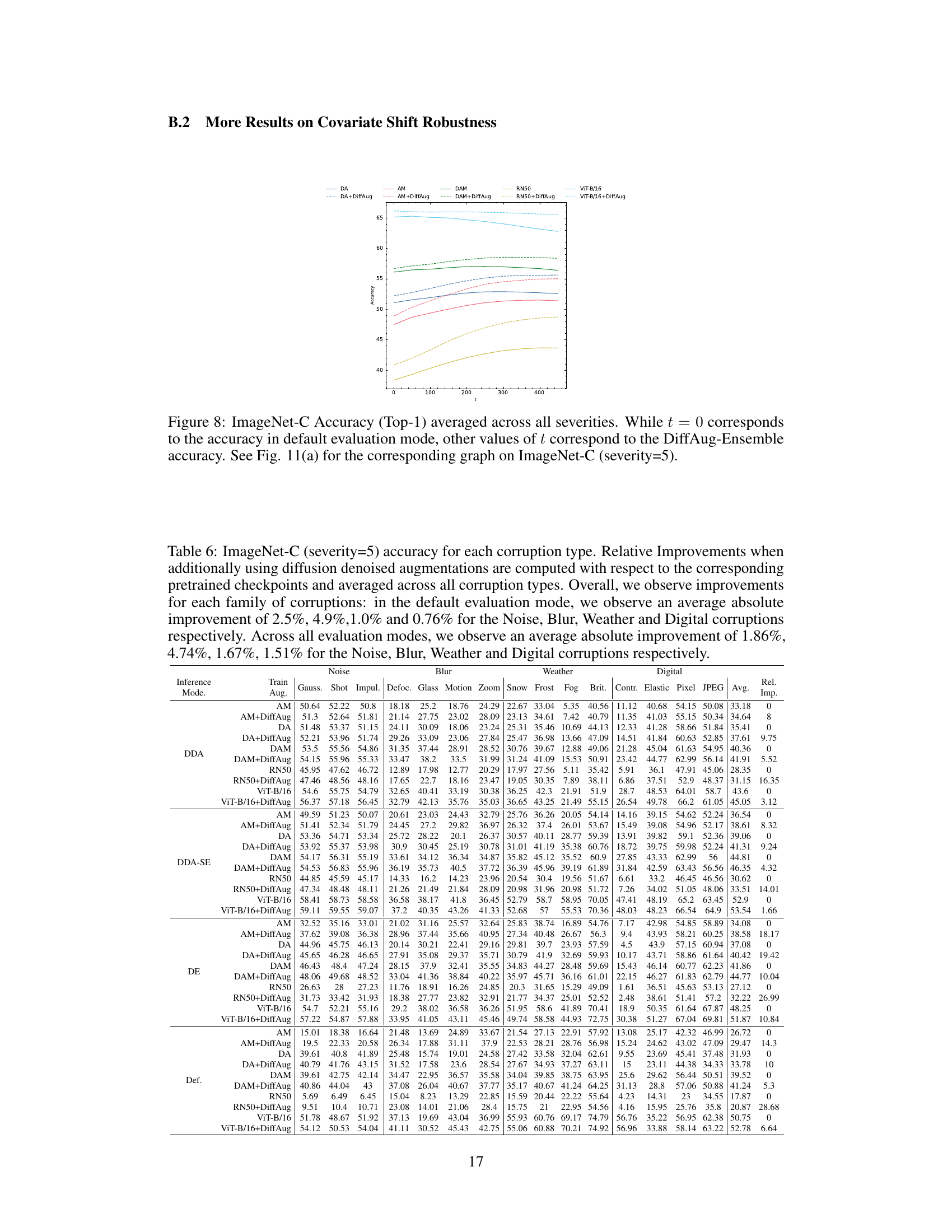
🔼 The figure shows the accuracy of the DiffAug Ensemble (DE) method on the ImageNet-C dataset (severity 5) for different step sizes in the range of diffusion times. The x-axis represents the diffusion time t, and the y-axis represents the accuracy. Different colors represent different augmentation methods (DA, AM, DAM, ViT-B/16, and RN50). The top row shows results for the base models, and the bottom row shows results with DiffAug applied. The figure demonstrates that the DE method’s accuracy is relatively consistent across different step sizes, although a step size of 25 tends to result in slightly better accuracy.
read the caption
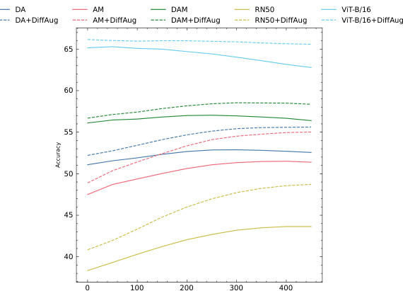
Figure 12: Plots of t vs DE Accuracy on Imagenet-C (severity=5) for different step-sizes: in general, we observe that the performance is largely robust to the choice of step-size although using t = 25 gives slightly improved result.

🔼 The figure shows the accuracy of the DiffAug Ensemble (DE) method on the ImageNet-C dataset with a severity of 5, for different step sizes (25, 50, and 75) of the diffusion process. The x-axis represents the diffusion time t, and the y-axis represents the accuracy. The plot shows that the performance of DE is relatively consistent across different step sizes, with a slight improvement observed for step size 25. This suggests that the DE method is robust to variations in the sampling parameters of the diffusion process.
read the caption
Figure 12: Plots of t vs DE Accuracy on Imagenet-C (severity=5) for different step-sizes: in general, we observe that the performance is largely robust to the choice of step-size although using t = 25 gives slightly improved result.
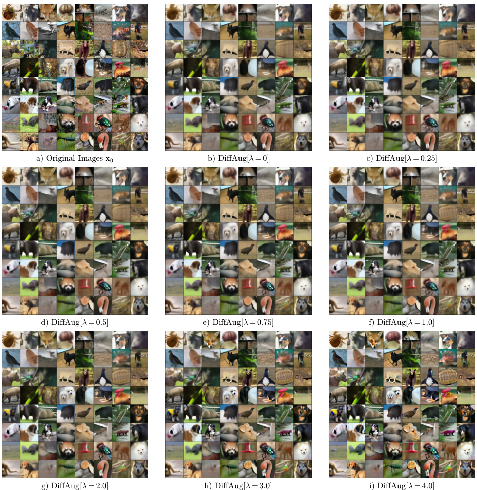
🔼 This figure shows a qualitative comparison of the DiffAug augmentations generated using various values of lambda (λ) at a fixed diffusion time t = 600. It demonstrates how altering the balance between unconditional and conditional score functions affects the augmentations generated by DiffAug. Each row represents a different value of λ, with the original images in the first column and augmented images in subsequent columns.
read the caption
Figure 14: We illustrate the DiffAug augmentations for various values of λ at t = 600.
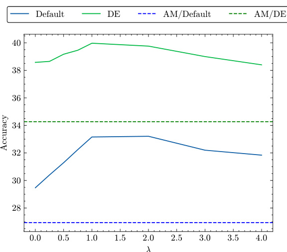
🔼 This figure shows the ImageNet-C accuracy (severity 5) for different values of lambda (λ). It compares the performance of the default method, DiffAug Ensemble (DE), AugMix with the default method, and AugMix with DE. The results demonstrate that conditional DiffAug can improve accuracy with optimal lambda values, but also that DiffAug can be effective with unconditional diffusion models, increasing its applicability.
read the caption
Figure 15: We extend AugMix(AM) with DiffAug using different values of λ and plot the ImageNet-C (severity=5) accuracy for both default and DE inference. We observe that conditional DiffAug can enhance performance for optimal values of λ. Nevertheless, DiffAug can also be applied with unconditional diffusion models broadening its applications.
🔼 This figure shows how DiffAug generates augmentations of training images. It starts with four original images (x0) and shows 8 augmented versions (xt) for each original image using different diffusion times (t). The augmentations where t is closer to 0 are more similar to the original while augmentations at larger t values introduce noise and are less similar to the originals. Interestingly, this noise does not negatively impact classifier accuracy but makes them more robust.
read the caption
Figure 1: DiffAug Augmentations. The leftmost column shows four original training examples (x0); to the right of that, we display 8 random augmentations (xt) for each image between t = 350 and t = 700 in steps of size 50. Augmentations generated for t < 350 are closer to the input image while the augmentations for t > 700 are farther from the input image. We observe that the diffusion denoised augmentations with larger values of t do not preserve the class label introducing noise in the training procedure. However, we find that this does not lead to empirical degradation of classification accuracy but instead contributes to improved robustness. Also, see Fig. 6 in appendix for a toy 2d example.
🔼 This figure shows examples of augmentations generated using DiffAug. The leftmost column displays four original training images. The remaining columns show eight augmented versions of each original image, created by diffusing the original image to various time steps (t) between 350 and 700 and then applying a single-step denoising. The augmentations become increasingly different from the originals as time t increases. Although the augmentations for larger t may not perfectly maintain the original class labels, this does not negatively impact classification accuracy and surprisingly improves robustness.
read the caption
Figure 1: DiffAug Augmentations. The leftmost column shows four original training examples (x0); to the right of that, we display 8 random augmentations (xt) for each image between t = 350 and t = 700 in steps of size 50. Augmentations generated for t < 350 are closer to the input image while the augmentations for t > 700 are farther from the input image. We observe that the diffusion denoised augmentations with larger values of t do not preserve the class label introducing noise in the training procedure. However, we find that this does not lead to empirical degradation of classification accuracy but instead contributes to improved robustness. Also, see Fig. 6 in appendix for a toy 2d example.

🔼 This figure shows the effect of DiffAug on four example images. The leftmost column displays the original images. The following columns show augmentations of those images generated by DiffAug at different time steps (t). Augmentations at lower time steps (closer to 0) are more similar to the original images, while higher time steps (closer to T) are more noisy and less visually similar. The important observation is that despite the introduction of noise in higher time steps, the classification accuracy does not degrade and even improves. This is attributed to a regularization effect from DiffAug that enhances the robustness of the classifier.
read the caption
Figure 1: DiffAug Augmentations. The leftmost column shows four original training examples (x0); to the right of that, we display 8 random augmentations (xt) for each image between t = 350 and t = 700 in steps of size 50. Augmentations generated for t < 350 are closer to the input image while the augmentations for t > 700 are farther from the input image. We observe that the diffusion denoised augmentations with larger values of t do not preserve the class label introducing noise in the training procedure. However, we find that this does not lead to empirical degradation of classification accuracy but instead contributes to improved robustness. Also, see Fig. 6 in appendix for a toy 2d example.

🔼 This figure shows examples of augmentations generated using DiffAug. Four original images are shown, along with 8 augmentations for each using different diffusion times (t). As t increases, the augmentations become more different from the original images, and the class label is sometimes changed. Despite this, the authors find that including these noisy augmentations actually improves the robustness of the resulting classifier, rather than degrading accuracy.
read the caption
Figure 1: DiffAug Augmentations. The leftmost column shows four original training examples (x0); to the right of that, we display 8 random augmentations (xt) for each image between t = 350 and t = 700 in steps of size 50. Augmentations generated for t < 350 are closer to the input image while the augmentations for t > 700 are farther from the input image. We observe that the diffusion denoised augmentations with larger values of t do not preserve the class label introducing noise in the training procedure. However, we find that this does not lead to empirical degradation of classification accuracy but instead contributes to improved robustness. Also, see Fig. 6 in appendix for a toy 2d example.

🔼 This figure shows examples of augmentations generated using the DiffAug method. The leftmost column displays four original training images. The following columns show eight augmentations of each image at various diffusion times (t) ranging from 350 to 700. As time increases, the augmentations become increasingly different from the original images, introducing noise. However, this noise surprisingly does not negatively affect the accuracy, suggesting a regularizing effect which enhances robustness.
read the caption
Figure 1: DiffAug Augmentations. The leftmost column shows four original training examples (x0); to the right of that, we display 8 random augmentations (xt) for each image between t = 350 and t = 700 in steps of size 50. Augmentations generated for t < 350 are closer to the input image while the augmentations for t > 700 are farther from the input image. We observe that the diffusion denoised augmentations with larger values of t do not preserve the class label introducing noise in the training procedure. However, we find that this does not lead to empirical degradation of classification accuracy but instead contributes to improved robustness. Also, see Fig. 6 in appendix for a toy 2d example.
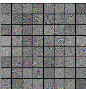
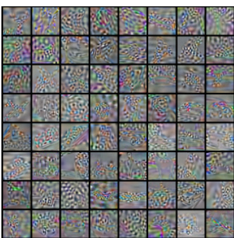
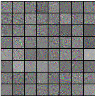
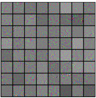
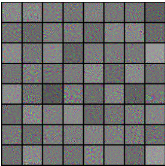
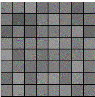
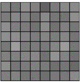
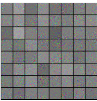
🔼 This figure shows the columns of the matrix U obtained from applying SVD decomposition to the Jacobian matrix J. Each image represents a principal component of the transformation applied by the denoising step in DiffAug. The average eigenvalue for each component is displayed, indicating the relative importance of each principal component in capturing the variations in the image data.
read the caption
Figure 17: Columns of U
🔼 This figure shows the effect of DiffAug on four example images. The leftmost column displays the original images. The remaining columns show augmentations generated by DiffAug at different timesteps (t). As t increases, the augmentations become noisier and less similar to the original image. Interestingly, the authors found that even though augmentations at higher values of t lose the original class label, it improved the classifier’s robustness, rather than degrading its accuracy.
read the caption
Figure 1: DiffAug Augmentations. The leftmost column shows four original training examples (x0); to the right of that, we display 8 random augmentations (xˆt) for each image between t = 350 and t = 700 in steps of size 50. Augmentations generated for t < 350 are closer to the input image while the augmentations for t > 700 are farther from the input image. We observe that the diffusion denoised augmentations with larger values of t do not preserve the class label introducing noise in the training procedure. However, we find that this does not lead to empirical degradation of classification accuracy but instead contributes to improved robustness. Also, see Fig. 6 in appendix for a toy 2d example.

🔼 This figure shows examples of augmentations generated by DiffAug. The leftmost column displays four original training images. The remaining columns show 8 augmentations of each original image for different diffusion times (t). As t increases, the augmentations become increasingly noisy and deviate from the original image. Importantly, even though some augmentations at larger t values change the class label (introducing noise), the overall classification accuracy is not negatively affected; this illustrates the robustness-improving properties of DiffAug. A simplified example in a 2D space is also available in Figure 6 of the appendix.
read the caption
Figure 1: DiffAug Augmentations. The leftmost column shows four original training examples (x0); to the right of that, we display 8 random augmentations (xt) for each image between t = 350 and t = 700 in steps of size 50. Augmentations generated for t < 350 are closer to the input image while the augmentations for t > 700 are farther from the input image. We observe that the diffusion denoised augmentations with larger values of t do not preserve the class label introducing noise in the training procedure. However, we find that this does not lead to empirical degradation of classification accuracy but instead contributes to improved robustness. Also, see Fig. 6 in appendix for a toy 2d example.

🔼 This figure shows examples of augmentations generated using the DiffAug technique. The leftmost column displays four original training images. The following columns show eight augmentations of each original image generated with different diffusion times (t). As t increases, the augmentations become increasingly noisy and less visually similar to the original images. The caption notes a surprising observation that these noisy augmentations, despite not preserving the class label in some cases, do not harm classifier performance and can even improve robustness.
read the caption
Figure 1: DiffAug Augmentations. The leftmost column shows four original training examples (x0); to the right of that, we display 8 random augmentations (xt) for each image between t = 350 and t = 700 in steps of size 50. Augmentations generated for t < 350 are closer to the input image while the augmentations for t > 700 are farther from the input image. We observe that the diffusion denoised augmentations with larger values of t do not preserve the class label introducing noise in the training procedure. However, we find that this does not lead to empirical degradation of classification accuracy but instead contributes to improved robustness. Also, see Fig. 6 in appendix for a toy 2d example.

🔼 This figure shows the effect of DiffAug on four example images. The leftmost column displays the original images. The remaining columns show augmentations of each original image generated using DiffAug with different values of the diffusion time, t. As t increases, the augmentations become more noisy and less visually similar to the original image. Interestingly, despite introducing label noise for larger t values, the process improves classifier robustness.
read the caption
Figure 1: DiffAug Augmentations. The leftmost column shows four original training examples (x0); to the right of that, we display 8 random augmentations (xt) for each image between t = 350 and t = 700 in steps of size 50. Augmentations generated for t < 350 are closer to the input image while the augmentations for t > 700 are farther from the input image. We observe that the diffusion denoised augmentations with larger values of t do not preserve the class label introducing noise in the training procedure. However, we find that this does not lead to empirical degradation of classification accuracy but instead contributes to improved robustness. Also, see Fig. 6 in appendix for a toy 2d example.
🔼 This figure shows how DiffAug generates augmentations of training images. It shows four original images and their corresponding augmentations at different diffusion times (t). Augmentations with smaller t values are visually similar to the originals, while augmentations with larger t values are more distorted. The key takeaway is that even though the augmentations with larger t values introduce class label noise, they surprisingly improve the robustness of the trained classifier.
read the caption
Figure 1: DiffAug Augmentations. The leftmost column shows four original training examples (x0); to the right of that, we display 8 random augmentations (xt) for each image between t = 350 and t = 700 in steps of size 50. Augmentations generated for t < 350 are closer to the input image while the augmentations for t > 700 are farther from the input image. We observe that the diffusion denoised augmentations with larger values of t do not preserve the class label introducing noise in the training procedure. However, we find that this does not lead to empirical degradation of classification accuracy but instead contributes to improved robustness. Also, see Fig. 6 in appendix for a toy 2d example.
🔼 This figure shows examples of augmentations generated using the DiffAug technique. The leftmost column displays the original images, while the other columns show variations created by diffusing the original image and then applying a single step of reverse diffusion. The augmentations range from subtle changes (near original image) to significant alterations (far from the original). Importantly, it shows that while some augmentations change the class label of the image, this does not negatively impact classifier accuracy but enhances robustness. The figure illustrates the impact of the time parameter (t) on the degree of augmentation applied.
read the caption
Figure 1: DiffAug Augmentations. The leftmost column shows four original training examples (x0); to the right of that, we display 8 random augmentations (xt) for each image between t = 350 and t = 700 in steps of size 50. Augmentations generated for t < 350 are closer to the input image while the augmentations for t > 700 are farther from the input image. We observe that the diffusion denoised augmentations with larger values of t do not preserve the class label introducing noise in the training procedure. However, we find that this does not lead to empirical degradation of classification accuracy but instead contributes to improved robustness. Also, see Fig. 6 in appendix for a toy 2d example.
🔼 This figure shows how DiffAug affects training images. The leftmost column displays four original images. The remaining columns show eight augmented versions of each original image, created using different levels of noise (represented by the variable ’t’). Images with lower ’t’ values are similar to the originals, while those with higher ’t’ values look quite different and may have their class labels altered, implying that the added noise acts as a regularizer for the training process.
read the caption
Figure 1: DiffAug Augmentations. The leftmost column shows four original training examples (x0); to the right of that, we display 8 random augmentations (xt) for each image between t = 350 and t = 700 in steps of size 50. Augmentations generated for t < 350 are closer to the input image while the augmentations for t > 700 are farther from the input image. We observe that the diffusion denoised augmentations with larger values of t do not preserve the class label introducing noise in the training procedure. However, we find that this does not lead to empirical degradation of classification accuracy but instead contributes to improved robustness. Also, see Fig. 6 in appendix for a toy 2d example.
🔼 This figure shows examples of augmentations generated using DiffAug. The leftmost column contains four original training examples. The remaining columns show eight augmentations of each original image, generated at various diffusion times (t). As t increases, the augmentations become increasingly noisy and less visually similar to the original, showing how DiffAug introduces noise in training. Despite this, the study discovered that the accuracy doesn’t decrease but rather improves robustness.
read the caption
Figure 1: DiffAug Augmentations. The leftmost column shows four original training examples (x0); to the right of that, we display 8 random augmentations (xt) for each image between t = 350 and t = 700 in steps of size 50. Augmentations generated for t < 350 are closer to the input image while the augmentations for t > 700 are farther from the input image. We observe that the diffusion denoised augmentations with larger values of t do not preserve the class label introducing noise in the training procedure. However, we find that this does not lead to empirical degradation of classification accuracy but instead contributes to improved robustness. Also, see Fig. 6 in appendix for a toy 2d example.
🔼 This figure shows examples of augmentations generated by DiffAug for four different images. DiffAug involves a forward diffusion step (adding noise) followed by a single reverse diffusion step (denoising). The figure demonstrates how the augmentations change as the diffusion time t varies. Augmentations with lower t values are similar to the originals, while those with higher t values are significantly noisier and sometimes appear to change class label. The authors found that this injection of noise into the training data surprisingly improved model robustness.
read the caption
Figure 1: DiffAug Augmentations. The leftmost column shows four original training examples (x0); to the right of that, we display 8 random augmentations (xt) for each image between t = 350 and t = 700 in steps of size 50. Augmentations generated for t < 350 are closer to the input image while the augmentations for t > 700 are farther from the input image. We observe that the diffusion denoised augmentations with larger values of t do not preserve the class label introducing noise in the training procedure. However, we find that this does not lead to empirical degradation of classification accuracy but instead contributes to improved robustness. Also, see Fig. 6 in appendix for a toy 2d example.
🔼 This figure shows examples of augmentations generated using DiffAug. The leftmost column displays four original training images. To the right, eight augmented versions of each image are shown, generated using different diffusion times (t) ranging from 350 to 700. The augmentation process involves a forward diffusion step followed by a single reverse diffusion step. Images with smaller t values look more like the originals, while those with higher t values are more heavily distorted. Notably, some augmented images have changed class labels, demonstrating the introduction of noise that surprisingly enhances robustness in the training process.
read the caption
Figure 1: DiffAug Augmentations. The leftmost column shows four original training examples (x0); to the right of that, we display 8 random augmentations (xt) for each image between t = 350 and t = 700 in steps of size 50. Augmentations generated for t < 350 are closer to the input image while the augmentations for t > 700 are farther from the input image. We observe that the diffusion denoised augmentations with larger values of t do not preserve the class label introducing noise in the training procedure. However, we find that this does not lead to empirical degradation of classification accuracy but instead contributes to improved robustness. Also, see Fig. 6 in appendix for a toy 2d example.

🔼 This figure shows examples of augmentations generated by DiffAug, a diffuse-and-denoise augmentation technique. Four original images are shown alongside eight augmentations for each image, generated at different time steps (t) during the reverse diffusion process. As t increases, the augmentations become more different from the original images and less likely to preserve the class label; however, surprisingly, this does not harm the classifier’s accuracy and improves its robustness.
read the caption
Figure 1: DiffAug Augmentations. The leftmost column shows four original training examples (x0); to the right of that, we display 8 random augmentations (xt) for each image between t = 350 and t = 700 in steps of size 50. Augmentations generated for t < 350 are closer to the input image while the augmentations for t > 700 are farther from the input image. We observe that the diffusion denoised augmentations with larger values of t do not preserve the class label introducing noise in the training procedure. However, we find that this does not lead to empirical degradation of classification accuracy but instead contributes to improved robustness. Also, see Fig. 6 in appendix for a toy 2d example.
🔼 This figure shows examples of augmentations generated using the DiffAug method. The leftmost column displays four original images. The remaining columns show eight augmented versions of each original image, created by varying the diffusion time parameter (t) from 350 to 700. As t increases, the augmentation becomes increasingly different from the original, highlighting that some augmentations may even lose their original class label. The paper argues that despite this, DiffAug improves robustness.
read the caption
Figure 1: DiffAug Augmentations. The leftmost column shows four original training examples (x0); to the right of that, we display 8 random augmentations (xt) for each image between t = 350 and t = 700 in steps of size 50. Augmentations generated for t < 350 are closer to the input image while the augmentations for t > 700 are farther from the input image. We observe that the diffusion denoised augmentations with larger values of t do not preserve the class label introducing noise in the training procedure. However, we find that this does not lead to empirical degradation of classification accuracy but instead contributes to improved robustness. Also, see Fig. 6 in appendix for a toy 2d example.

🔼 This figure shows examples of augmentations generated by DiffAug, a new technique introduced in the paper for training robust classifiers. The figure displays four original images and eight augmented versions for each, showing how the augmentation process progressively introduces noise as time (t) increases. Despite adding noise that changes class labels in some cases, these augmentations do not negatively impact the classifier’s accuracy, but instead improve its robustness.
read the caption
Figure 1: DiffAug Augmentations. The leftmost column shows four original training examples (x0); to the right of that, we display 8 random augmentations (xt) for each image between t = 350 and t = 700 in steps of size 50. Augmentations generated for t < 350 are closer to the input image while the augmentations for t > 700 are farther from the input image. We observe that the diffusion denoised augmentations with larger values of t do not preserve the class label introducing noise in the training procedure. However, we find that this does not lead to empirical degradation of classification accuracy but instead contributes to improved robustness. Also, see Fig. 6 in appendix for a toy 2d example.
🔼 This figure shows the effect of DiffAug on four example images. The leftmost column shows the original images. The following columns show augmentations generated using different diffusion times (t). As t increases, the augmentations become noisier and less similar to the original image. Notably, even with significant noise, the augmentations do not negatively impact the classification accuracy, suggesting a regularization effect.
read the caption
Figure 1: DiffAug Augmentations. The leftmost column shows four original training examples (x0); to the right of that, we display 8 random augmentations (xt) for each image between t = 350 and t = 700 in steps of size 50. Augmentations generated for t < 350 are closer to the input image while the augmentations for t > 700 are farther from the input image. We observe that the diffusion denoised augmentations with larger values of t do not preserve the class label introducing noise in the training procedure. However, we find that this does not lead to empirical degradation of classification accuracy but instead contributes to improved robustness. Also, see Fig. 6 in appendix for a toy 2d example.
🔼 This figure shows examples of augmentations generated using the DiffAug method. The leftmost column displays four original training images. The remaining columns illustrate eight augmented versions of each original image, created by applying DiffAug with different diffusion times (t) ranging from 350 to 700. The augmentations become increasingly noisy as t increases, with some even losing their original class label. Despite this, the authors observed improved robustness in classifiers trained with these augmentations.
read the caption
Figure 1: DiffAug Augmentations. The leftmost column shows four original training examples (x0); to the right of that, we display 8 random augmentations (xt) for each image between t = 350 and t = 700 in steps of size 50. Augmentations generated for t < 350 are closer to the input image while the augmentations for t > 700 are farther from the input image. We observe that the diffusion denoised augmentations with larger values of t do not preserve the class label introducing noise in the training procedure. However, we find that this does not lead to empirical degradation of classification accuracy but instead contributes to improved robustness. Also, see Fig. 6 in appendix for a toy 2d example.
🔼 This figure shows the effect of DiffAug on four example images. The leftmost column shows the original images. The remaining columns show eight augmented versions of each image created using different diffusion times (t) ranging from 350 to 700. As t increases, the augmentations become increasingly different from the original images, introducing noise. Notably, despite this noise, the augmentations still maintain enough information for the classifier to learn, resulting in improved robustness.
read the caption
Figure 1: DiffAug Augmentations. The leftmost column shows four original training examples (x0); to the right of that, we display 8 random augmentations (xt) for each image between t = 350 and t = 700 in steps of size 50. Augmentations generated for t < 350 are closer to the input image while the augmentations for t > 700 are farther from the input image. We observe that the diffusion denoised augmentations with larger values of t do not preserve the class label introducing noise in the training procedure. However, we find that this does not lead to empirical degradation of classification accuracy but instead contributes to improved robustness. Also, see Fig. 6 in appendix for a toy 2d example.

🔼 This figure shows examples of augmentations generated by DiffAug. The leftmost column shows original images. The rest show how the same image is transformed using different diffusion times (t). As t increases, the resulting image increasingly deviates from the original but the class label is maintained, surprisingly improving the robustness of the model.
read the caption
Figure 1: DiffAug Augmentations. The leftmost column shows four original training examples (x0); to the right of that, we display 8 random augmentations (xt) for each image between t = 350 and t = 700 in steps of size 50. Augmentations generated for t < 350 are closer to the input image while the augmentations for t > 700 are farther from the input image. We observe that the diffusion denoised augmentations with larger values of t do not preserve the class label introducing noise in the training procedure. However, we find that this does not lead to empirical degradation of classification accuracy but instead contributes to improved robustness. Also, see Fig. 6 in appendix for a toy 2d example.
🔼 This figure shows how DiffAug generates augmentations of training images. It starts with an original image (x0) and applies a forward diffusion step to introduce noise, followed by a reverse diffusion step (denoising). The results (xt) are shown for various levels of noise (t values). While higher noise levels introduce a degree of label noise, this doesn’t hurt accuracy but improves robustness. The figure illustrates this concept with several examples. A simplified 2D representation is also available in the appendix.
read the caption
Figure 1: DiffAug Augmentations. The leftmost column shows four original training examples (x0); to the right of that, we display 8 random augmentations (xt) for each image between t = 350 and t = 700 in steps of size 50. Augmentations generated for t < 350 are closer to the input image while the augmentations for t > 700 are farther from the input image. We observe that the diffusion denoised augmentations with larger values of t do not preserve the class label introducing noise in the training procedure. However, we find that this does not lead to empirical degradation of classification accuracy but instead contributes to improved robustness. Also, see Fig. 6 in appendix for a toy 2d example.
🔼 This figure shows examples of augmentations generated using the DiffAug method. It displays four original training images and eight augmentations for each. The augmentations vary in their level of noise, which is controlled by a time parameter (t). While higher noise levels (larger t) can lead to some loss of original label information, this doesn’t negatively impact the model’s overall accuracy and actually seems to improve robustness.
read the caption
Figure 1: DiffAug Augmentations. The leftmost column shows four original training examples (x0); to the right of that, we display 8 random augmentations (xt) for each image between t = 350 and t = 700 in steps of size 50. Augmentations generated for t < 350 are closer to the input image while the augmentations for t > 700 are farther from the input image. We observe that the diffusion denoised augmentations with larger values of t do not preserve the class label introducing noise in the training procedure. However, we find that this does not lead to empirical degradation of classification accuracy but instead contributes to improved robustness. Also, see Fig. 6 in appendix for a toy 2d example.
🔼 This figure shows examples of augmentations generated using DiffAug. The leftmost column displays four original training images. The remaining columns show 8 augmented versions of each original image, produced by diffusing the images to different time steps (t) in a diffusion process and then applying a single denoising step. The augmentations range from very similar to the original (t close to 0) to very different (t close to 700). Although the larger t values sometimes change the class label, this noise surprisingly improves classifier robustness.
read the caption
Figure 1: DiffAug Augmentations. The leftmost column shows four original training examples (x0); to the right of that, we display 8 random augmentations (xt) for each image between t = 350 and t = 700 in steps of size 50. Augmentations generated for t < 350 are closer to the input image while the augmentations for t > 700 are farther from the input image. We observe that the diffusion denoised augmentations with larger values of t do not preserve the class label introducing noise in the training procedure. However, we find that this does not lead to empirical degradation of classification accuracy but instead contributes to improved robustness. Also, see Fig. 6 in appendix for a toy 2d example.
🔼 This figure demonstrates the effect of DiffAug on four example images. It shows the original images (x0) and 8 augmented versions (xt) for each image. The augmentations are generated by applying a forward diffusion step followed by a reverse diffusion step for different time steps (t). Augmentations with small t values look similar to the original image, while large t values create images that are quite different. This shows that even though the class label might not be preserved during the augmentation with larger t, the overall classification performance doesn’t degrade and actually improves.
read the caption
Figure 1: DiffAug Augmentations. The leftmost column shows four original training examples (x0); to the right of that, we display 8 random augmentations (xt) for each image between t = 350 and t = 700 in steps of size 50. Augmentations generated for t < 350 are closer to the input image while the augmentations for t > 700 are farther from the input image. We observe that the diffusion denoised augmentations with larger values of t do not preserve the class label introducing noise in the training procedure. However, we find that this does not lead to empirical degradation of classification accuracy but instead contributes to improved robustness. Also, see Fig. 6 in appendix for a toy 2d example.
🔼 This figure shows the effect of DiffAug on four example images. The leftmost column shows the original images. The remaining columns show eight augmented versions of each image, generated using DiffAug with different diffusion times (t). The augmentations with smaller t values are similar to the original image while larger t values result in augmented images that are significantly different. Interestingly, the images with larger t values, which introduce class label noise, do not hurt the classifier’s performance but actually improve robustness.
read the caption
Figure 1: DiffAug Augmentations. The leftmost column shows four original training examples (x0); to the right of that, we display 8 random augmentations (xt) for each image between t = 350 and t = 700 in steps of size 50. Augmentations generated for t < 350 are closer to the input image while the augmentations for t > 700 are farther from the input image. We observe that the diffusion denoised augmentations with larger values of t do not preserve the class label introducing noise in the training procedure. However, we find that this does not lead to empirical degradation of classification accuracy but instead contributes to improved robustness. Also, see Fig. 6 in appendix for a toy 2d example.
🔼 This figure shows examples of augmentations generated using the DiffAug method. Four original images are shown alongside 8 augmentations of each, created by diffusing the original image to different points in time (t) and then performing a single denoising step. The augmentations closer to the original image (lower t) preserve the class label better, whilst augmentations that are further from the original image (higher t) do not preserve the class label. Interestingly, this injection of label noise does not appear to negatively impact the model’s overall performance and may contribute to improved robustness.
read the caption
Figure 1: DiffAug Augmentations. The leftmost column shows four original training examples (x0); to the right of that, we display 8 random augmentations (xt) for each image between t = 350 and t = 700 in steps of size 50. Augmentations generated for t < 350 are closer to the input image while the augmentations for t > 700 are farther from the input image. We observe that the diffusion denoised augmentations with larger values of t do not preserve the class label introducing noise in the training procedure. However, we find that this does not lead to empirical degradation of classification accuracy but instead contributes to improved robustness. Also, see Fig. 6 in appendix for a toy 2d example.
🔼 This figure shows how the DiffAug augmentation technique works. Four original images are shown in the leftmost column. For each of these images, eight augmented versions are shown, generated using different diffusion times (t). The augmentations generated with smaller diffusion times (t < 350) are very similar to the original images, while those with larger diffusion times (t > 700) look very different. Even though the augmentations with large t values may change the class label, this does not appear to negatively impact classifier accuracy and may even enhance robustness.
read the caption
Figure 1: DiffAug Augmentations. The leftmost column shows four original training examples (x0); to the right of that, we display 8 random augmentations (xt) for each image between t = 350 and t = 700 in steps of size 50. Augmentations generated for t < 350 are closer to the input image while the augmentations for t > 700 are farther from the input image. We observe that the diffusion denoised augmentations with larger values of t do not preserve the class label introducing noise in the training procedure. However, we find that this does not lead to empirical degradation of classification accuracy but instead contributes to improved robustness. Also, see Fig. 6 in appendix for a toy 2d example.
🔼 This figure shows how DiffAug generates augmentations of training examples. It takes an original image and applies a forward diffusion step followed by a reverse diffusion step. The figure displays eight augmentations for four original images, varying the time parameter (t) of diffusion. For smaller t, augmentations are visually similar to the original image, whereas larger t results in augmentations that differ significantly from the original and may even change class labels. However, this ’noise’ introduced through larger t improves robustness without significantly harming classification accuracy.
read the caption
Figure 1: DiffAug Augmentations. The leftmost column shows four original training examples (x0); to the right of that, we display 8 random augmentations (xt) for each image between t = 350 and t = 700 in steps of size 50. Augmentations generated for t < 350 are closer to the input image while the augmentations for t > 700 are farther from the input image. We observe that the diffusion denoised augmentations with larger values of t do not preserve the class label introducing noise in the training procedure. However, we find that this does not lead to empirical degradation of classification accuracy but instead contributes to improved robustness. Also, see Fig. 6 in appendix for a toy 2d example.
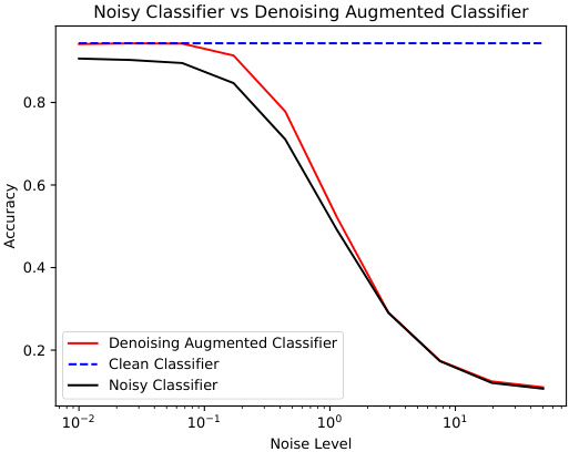
🔼 This figure shows the test accuracy of three CIFAR10 classifiers against different noise levels. The ‘Clean Classifier’ represents the baseline model trained on clean data. The ‘Noisy Classifier’ is trained on noisy images as input and serves as a comparative baseline. The ‘Denoising Augmented Classifier’ uses both the noisy and the denoised images as input during training.
read the caption
Figure 19: CIFAR10: Test Accuracy vs. Noise Scale.
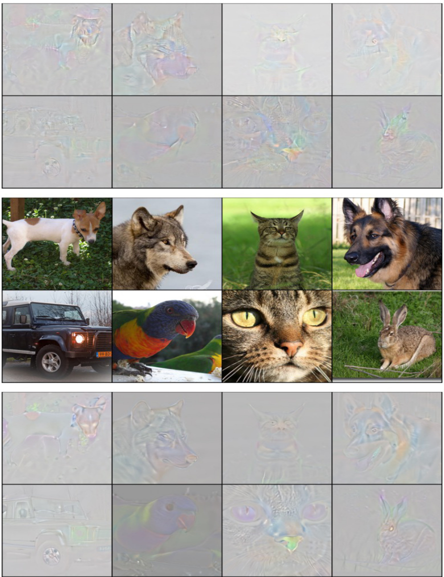
🔼 This figure shows examples of perceptually aligned gradients (PAGs) obtained using the Vision Transformer (ViT) architecture trained with DiffAug. The left column shows original Imagenet images. The right column displays the min-max normalized gradients for these images after they have been diffused to time step t=300. Contrast maximization is applied to enhance the visualization of these gradients. The figure demonstrates that the gradients are aligned with human perception, indicating that the model is robust and has learned meaningful visual features.
read the caption
Figure 3: PAG example using ViT+DiffAug. We diffuse the Imagenet example (left) to t = 300 and visualise the min-max normalized classifier gradients (right). For easy viewing, we apply contrast maximization. More examples are shown below.

🔼 This figure shows a qualitative analysis of the classifier gradients obtained from one-step diffusion denoised examples using Vision Transformer (ViT) trained with DiffAug. The leftmost column displays original Imagenet examples. The middle column shows the examples after forward diffusion to t=300. The rightmost column shows the min-max normalized classifier gradients. Contrast maximization is applied for better visualization. The gradients exhibit perceptual alignment, meaning they align with human perception of the image features.
read the caption
Figure 3: PAG example using ViT+DiffAug. We diffuse the Imagenet example (left) to t = 300 and visualise the min-max normalized classifier gradients (right). For easy viewing, we apply contrast maximization. More examples are shown below.

🔼 This figure shows several examples of augmentations generated using the DiffAug technique. The leftmost column shows four original images. The rest of the columns show eight augmentations of each original image using different diffusion times (t). The augmentations are obtained by applying a forward diffusion step followed by a single reverse diffusion step. It is observed that when diffusion times are smaller, the augmented images are closer to the original images. When diffusion times are larger, the augmentations are farther from the original images and even change the class label. However, this does not seem to degrade classification accuracy and instead contributes to robustness.
read the caption
Figure 1: DiffAug Augmentations. The leftmost column shows four original training examples (x0); to the right of that, we display 8 random augmentations (xt) for each image between t = 350 and t = 700 in steps of size 50. Augmentations generated for t < 350 are closer to the input image while the augmentations for t > 700 are farther from the input image. We observe that the diffusion denoised augmentations with larger values of t do not preserve the class label introducing noise in the training procedure. However, we find that this does not lead to empirical degradation of classification accuracy but instead contributes to improved robustness. Also, see Fig. 6 in appendix for a toy 2d example.
🔼 This figure shows several examples of augmentations generated using the DiffAug method. The leftmost column shows original images, while the other columns display augmentations of those images at various levels of noise. The augmentations are created by applying a forward diffusion step followed by a reverse diffusion step using a diffusion model. The figure demonstrates that even though more noisy augmentations may not preserve the original class label, they do not negatively impact the overall classification accuracy and even improve robustness.
read the caption
Figure 1: DiffAug Augmentations. The leftmost column shows four original training examples (x0); to the right of that, we display 8 random augmentations (xt) for each image between t = 350 and t = 700 in steps of size 50. Augmentations generated for t < 350 are closer to the input image while the augmentations for t > 700 are farther from the input image. We observe that the diffusion denoised augmentations with larger values of t do not preserve the class label introducing noise in the training procedure. However, we find that this does not lead to empirical degradation of classification accuracy but instead contributes to improved robustness. Also, see Fig. 6 in appendix for a toy 2d example.
🔼 This figure shows examples of augmentations generated using the DiffAug method. The leftmost column displays four original training images. To the right, eight augmented versions of each original image are shown, created by varying the diffusion time parameter (t) between 350 and 700. Images with lower t values are similar to the originals, while those with higher t values differ significantly and even lose their original class labels. This illustrates that despite introducing label noise at high t values, DiffAug improves classifier robustness.
read the caption
Figure 1: DiffAug Augmentations. The leftmost column shows four original training examples (x0); to the right of that, we display 8 random augmentations (xt) for each image between t = 350 and t = 700 in steps of size 50. Augmentations generated for t < 350 are closer to the input image while the augmentations for t > 700 are farther from the input image. We observe that the diffusion denoised augmentations with larger values of t do not preserve the class label introducing noise in the training procedure. However, we find that this does not lead to empirical degradation of classification accuracy but instead contributes to improved robustness. Also, see Fig. 6 in appendix for a toy 2d example.
🔼 This figure shows examples of augmentations generated by DiffAug, the proposed diffusion-based augmentation technique. Four original images are shown alongside eight augmented versions of each, created by varying the diffusion time parameter (t). Early augmentations (small t) closely resemble the originals while later ones (large t) are highly noisy and visually dissimilar. Importantly, while these noisier augmentations can even change the class label, the experiment showed that they still improved the robustness of the classifier rather than decreasing accuracy.
read the caption
Figure 1: DiffAug Augmentations. The leftmost column shows four original training examples (x0); to the right of that, we display 8 random augmentations (xt) for each image between t = 350 and t = 700 in steps of size 50. Augmentations generated for t < 350 are closer to the input image while the augmentations for t > 700 are farther from the input image. We observe that the diffusion denoised augmentations with larger values of t do not preserve the class label introducing noise in the training procedure. However, we find that this does not lead to empirical degradation of classification accuracy but instead contributes to improved robustness. Also, see Fig. 6 in appendix for a toy 2d example.
More on tables

🔼 This table compares the top-1 accuracy of ResNet50 models trained with and without DiffAug and with and without additional synthetic data generated by Stable Diffusion. The accuracy is evaluated across various image corruption types (ImageNet-C), real-world corruptions (ImageNet-R), sketches (ImageNet-Sketch), and out-of-distribution examples (ImageNet-A, ImageNet-D, and ImageNet-S). The table demonstrates DiffAug’s effectiveness in improving robustness even when compared to models trained with additional synthetic data.
read the caption
Table 2: Top-1 Accuracy (%) across different types of distribution shifts when additional high-quality synthetic data from Stable-Diffusion is available (denoted by +Synth). We show the net improvement obtained by DiffAug training and DiffAug-Ensemble (DE) inference. For reference, we also include the results for the corresponding ResNet50 models without extra synthetic data.

🔼 This table presents the Area Under the Receiver Operating Characteristic curve (AUROC) for different OOD detection algorithms on the ImageNet Near-OOD detection task. The algorithms are AugMix (AM), AM+DiffAug, RN50, RN50+DiffAug. The AUROC is a measure of the classifier’s ability to distinguish between in-distribution and out-of-distribution samples. Higher AUROC values indicate better performance.
read the caption
Table 3: AUROC on Imagenet Near-OOD Detection.

🔼 This table summarizes the test accuracy results for CIFAR10 and ImageNet datasets. Two types of classifiers were used: Noisy Classifier and DA-Classifier. The Noisy Classifier uses only noisy inputs, while the DA-Classifier uses both noisy and denoised inputs. The results show that the DA-Classifier significantly outperforms the Noisy Classifier on both datasets, indicating the effectiveness of denoising-augmented training.
read the caption
Table 4: Summary of Test Accuracies for CIFAR10 and Imagenet: each test example is diffused to a random uniformly sampled diffusion time. Both classifiers are shown the same diffused example.

🔼 This table presents the top-1 accuracy of different models trained with various data augmentation methods on ImageNet-C (a corrupted version of ImageNet with severity level 5) and ImageNet-Test. The augmentation methods include AugMix (AM), DeepAugment (DA), AugMix+DeepAugment (DAM), and DiffAug (with and without combinations of the other methods). Evaluation modes include standard classification, Diffusion-based test-time adaptation (DDA), DDA with self-ensembling (DDA-SE), and DiffAug Ensemble (DE). The average accuracy across all evaluation modes is also provided for each classifier.
read the caption
Table 1: Top-1 Accuracy (%) on Imagenet-C (severity=5) and Imagenet-Test. We summarize the results for each combination of Train-augmentations and evaluation modes. The average (avg) accuracies for each classifier and evaluation mode is shown.
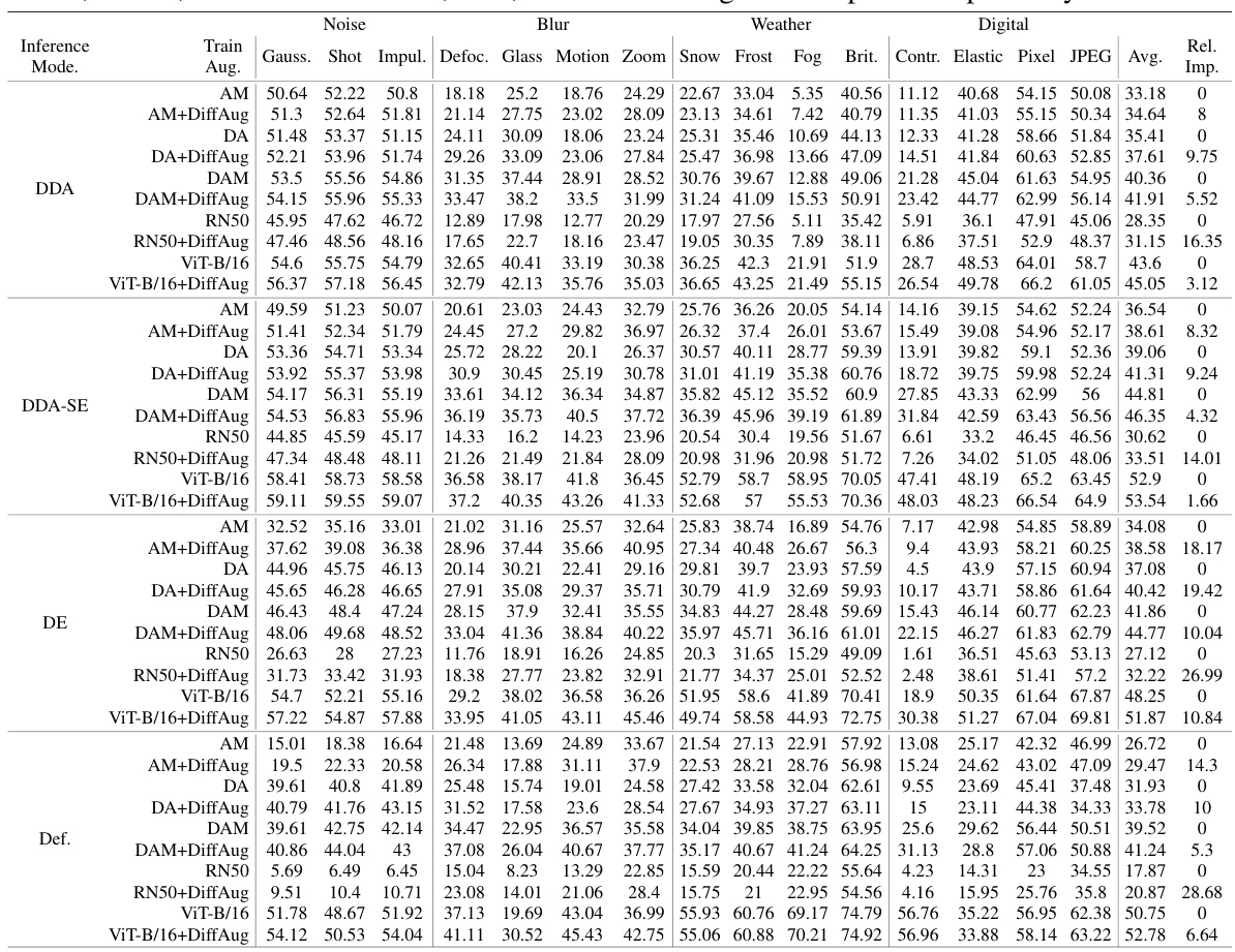
🔼 This table presents the ImageNet-C (severity=5) and ImageNet-Test top-1 accuracy results for various classifier training methods. It compares different augmentation strategies (AM, DA, DAM, and their combinations with DiffAug) and evaluation methods (DDA, DDA-SE, DE, and default). The average accuracy across different evaluation types is also included for each classifier and augmentation strategy.
read the caption
Table 1: Top-1 Accuracy (%) on Imagenet-C (severity=5) and Imagenet-Test. We summarize the results for each combination of Train-augmentations and evaluation modes. The average (avg) accuracies for each classifier and evaluation mode is shown.

🔼 This table presents the top-1 accuracy results on ImageNet-S and ImageNet-R datasets. It shows the performance of different classifier models trained with various augmentation techniques (including DiffAug) and evaluated under four different modes: DDA, DDA-SE, DE, and default. The average accuracy across all modes and augmentation techniques is also provided for each classifier model (ResNet-50 and ViT-B/16). This helps in comparing the robustness of different augmentation methods and classifier models on these datasets representing covariate shifts.
read the caption
Table 7: Top-1 Accuracy (%) on Imagenet-S and Imagenet-R. We summarize the results for each combination of Train-augmentations and evaluation modes. The average (avg) accuracies for each classifier and evaluation mode is shown.

🔼 This table presents the top-1 accuracy results on ImageNet-C (with severity level 5) and ImageNet-Test. It summarizes the performance of different classifier models trained with various augmentation techniques, including DiffAug. The table shows the accuracy for each model under different evaluation scenarios (Default, DDA, DDA-SE, and DE) and provides the average accuracy across these methods. The augmentation techniques used are AugMix (AM), DeepAugment (DA), DeepAugment+AugMix (DAM), and combinations with DiffAug.
read the caption
Table 1: Top-1 Accuracy (%) on Imagenet-C (severity=5) and Imagenet-Test. We summarize the results for each combination of Train-augmentations and evaluation modes. The average (avg) accuracies for each classifier and evaluation mode is shown.

🔼 This table presents the Top-1 accuracy results on ImageNet-C (with severity level 5) and ImageNet-Test datasets. It compares the performance of different classifier models trained with various augmentation techniques, including DiffAug and combinations with AugMix and DeepAugment. The results are categorized by evaluation method (DDA, DDA-SE, DE, and Default) to show robustness across different scenarios. The ‘Avg’ column provides an average across all augmentation methods for each evaluation type.
read the caption
Table 1: Top-1 Accuracy (%) on Imagenet-C (severity=5) and Imagenet-Test. We summarize the results for each combination of Train-augmentations and evaluation modes. The average (avg) accuracies for each classifier and evaluation mode is shown.

🔼 This table compares the average wall-clock time taken by DDA and DE for processing one image. The experiments used a 40GB A40 GPU. The maximum possible batch size was used for each method to obtain the reported average.
read the caption
Table 10: DDA vs DE in terms of wallclock times: We use 40GB A40 GPU for determining the running time. For each method, we determine the maximum usable batch-size and report the average wallclock time for processing a single example.

🔼 This table presents the ImageNet-C and ImageNet-Test top-1 accuracy for various classifier training methods and evaluation strategies (Default, DDA, DDA-SE, DE). The training methods combine different data augmentation techniques (AM, DA, DAM, DiffAug). The table shows how DiffAug improves the accuracy in multiple settings, and that the improvement is consistent across the different augmentation methods used.
read the caption
Table 1: Top-1 Accuracy (%) on Imagenet-C (severity=5) and Imagenet-Test. We summarize the results for each combination of Train-augmentations and evaluation modes. The average (avg) accuracies for each classifier and evaluation mode is shown.

🔼 This table compares the performance of DiffAug using different sampling methods (DDIM and DPM-Solver) for generating augmentations. The evaluation metric is top-1 accuracy on ImageNet-C (severity=5), and three different training methods are compared: AM (AugMix), AM+DiffAug/DDIM (AugMix with DiffAug using DDIM), and AM+DiffAug/DPM-Solver-2 (AugMix with DiffAug using DPM-Solver). The results show that using DDIM generally results in higher accuracy than using DPM-Solver for DiffAug augmentations.
read the caption
Table 12: Evaluation of other sampling methods for DiffAug: We use ↓ to denote lower performance due to the use of DPM-Solver instead of DDIM.

🔼 This table shows the certified accuracy for different l2 perturbation radius. The authors selected the best noise scale (σ) from a set of three (0.25, 0.5, 1.0) for each l2 radius to achieve the highest certified accuracy. The results are presented for two models: ViT and ViT trained with DiffAug (ViT+DiffAug).
read the caption
Table 13: Certified Accuracy for different l2 perturbation radius. As is standard in the literature, we consider σε ∈ {0.25, 0.5, 1.0} and select the best σε for each l2 radius.
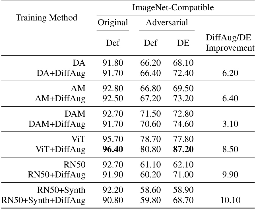
🔼 This table presents the ImageNet-C and ImageNet-Test top-1 accuracy results for various classifier training methods. The training methods combine different augmentation techniques (AugMix, DeepAugment, DiffAug) and evaluation methods (default, DDA, DDA-SE, DE). The table shows how different augmentation strategies affect the robustness of the classifiers and their performance on clean and corrupted images.
read the caption
Table 1: Top-1 Accuracy (%) on Imagenet-C (severity=5) and Imagenet-Test. We summarize the results for each combination of Train-augmentations and evaluation modes. The average (avg) accuracies for each classifier and evaluation mode is shown.

🔼 This table presents the top-1 accuracy of different models trained with various data augmentation techniques on the ImageNet-C dataset (with severity level 5) and the standard ImageNet-Test dataset. The augmentation techniques include AugMix (AM), DeepAugment (DA), AugMix+DeepAugment (DAM), and DiffAug, both independently and in combination with the others. The evaluation modes are standard classification, using the DDA image adaptation method, using DDA with self-ensembling, and DiffAug Ensemble (DE). The table shows the average accuracy across all these combinations for ResNet-50 and ViT models.
read the caption
Table 1: Top-1 Accuracy (%) on Imagenet-C (severity=5) and Imagenet-Test. We summarize the results for each combination of Train-augmentations and evaluation modes. The average (avg) accuracies for each classifier and evaluation mode is shown.

🔼 This table presents the top-1 accuracy results of different image classification models trained with various augmentation techniques on the ImageNet-C dataset (with a severity level of 5) and the standard ImageNet-Test dataset. The augmentation techniques include AugMix, DeepAugment, and their combinations with DiffAug. The evaluation modes encompass standard classification, as well as robustness evaluations using DDA, DDA-SE, and DE methods. The average accuracy across all models and evaluation methods is also provided for better comparison.
read the caption
Table 1: Top-1 Accuracy (%) on Imagenet-C (severity=5) and Imagenet-Test. We summarize the results for each combination of Train-augmentations and evaluation modes. The average (avg) accuracies for each classifier and evaluation mode is shown.

🔼 This table presents the ImageNet-C (severity=5) and ImageNet-Test top-1 accuracy for different classifier training methods. It compares several augmentation techniques, including AugMix (AM), DeepAugment (DA), and their combination (DAM), with and without the proposed DiffAug method. The evaluation includes standard classification accuracy, as well as robustness evaluation using three metrics: DDA (Diffusion-based test-time adaptation), DDA-SE (DDA with self-ensembling), and DE (DiffAug Ensemble). The table shows the average accuracy across all corruption types for each classifier and augmentation strategy, allowing comparison of the relative impact of each augmentation method on the overall performance.
read the caption
Table 1: Top-1 Accuracy (%) on Imagenet-C (severity=5) and Imagenet-Test. We summarize the results for each combination of Train-augmentations and evaluation modes. The average (avg) accuracies for each classifier and evaluation mode is shown.

🔼 This table presents the results of ImageNet Near-OOD detection experiments using various training augmentation techniques. The AUROC (Area Under the Receiver Operating Characteristic curve) and FPR@TPR95 (False Positive Rate at True Positive Rate of 95%) metrics are used to evaluate the out-of-distribution (OOD) detection performance of different models. The table compares the performance of models trained with different augmentations (AM, AM+DiffAug, RN50, RN50+DiffAug, DAM, DAM+DiffAug, DA, DA+DiffAug) across multiple OOD detection algorithms (ASH, MSP, ReAct, SCALE). The average performance across algorithms is also shown for each augmentation.
read the caption
Table 15: AUROC and FPR@TPR95 (lower is better) on ImageNet Near-OOD Detection.

🔼 This table presents the top-1 accuracy results on ImageNet-C (with a severity of 5) and ImageNet-Test. The results are broken down by different training augmentation methods (AM, DA, DAM, and their combinations with DiffAug), and by different evaluation methods (DDA, DDA-SE, DE, and the default method). It shows the impact of DiffAug on classification accuracy across various robustness evaluation scenarios.
read the caption
Table 1: Top-1 Accuracy (%) on Imagenet-C (severity=5) and Imagenet-Test. We summarize the results for each combination of Train-augmentations and evaluation modes. The average (avg) accuracies for each classifier and evaluation mode is shown.

🔼 This table presents the ImageNet-S and ImageNet-R Top-1 accuracy for different training augmentation methods. The results are broken down by evaluation method (DDA, DDA-SE, DE, Def.) to show the impact of different test-time augmentation strategies on model robustness across various datasets. The average accuracy across all methods is also provided for each classifier.
read the caption
Table 7: Top-1 Accuracy (%) on Imagenet-S and Imagenet-R. We summarize the results for each combination of Train-augmentations and evaluation modes. The average (avg) accuracies for each classifier and evaluation mode is shown.

🔼 This table presents the results of the ImageNet Near-OOD detection experiment. It shows the Area Under the Receiver Operating Characteristic curve (AUROC) and the False Positive Rate at 95% True Positive Rate (FPR@TPR95) for various OOD detection algorithms. The algorithms are evaluated using four different metrics: ASH, MSP, ReAct, and Scale. The table compares the performance of the models trained with AugMix (AM), AugMix combined with DiffAug (AM+DiffAug), AugMix combined with additional training (AM+Extra), AugMix combined with DiffAug using different time ranges (AM+DiffAug[0,500] and AM+DiffAug[500,999]). The average performance across all metrics is also presented for each model.
read the caption
Table 15: AUROC and FPR@TPR95 on ImageNet Near-OOD Detection.

🔼 This table presents the top-1 accuracy results of different classifiers trained with various augmentation methods on the ImageNet-C dataset (with severity level 5) and the standard ImageNet-Test dataset. It compares the performance using different test-time augmentation techniques (DDA, DDA-SE, DE, and default). The average accuracy across all methods is also provided for better comparison.
read the caption
Table 1: Top-1 Accuracy (%) on Imagenet-C (severity=5) and Imagenet-Test. We summarize the results for each combination of Train-augmentations and evaluation modes. The average (avg) accuracies for each classifier and evaluation mode is shown.

🔼 This table presents the top-1 accuracy results of different image classification models trained with various data augmentation techniques on the ImageNet-C dataset (with a severity level of 5) and the standard ImageNet test set. The augmentation techniques used include AugMix (AM), DeepAugment (DA), and a combination of both (DAM). The models are evaluated using different robustness evaluation methods including the standard accuracy as well as DDA, DDA-SE, and DE(DiffAug Ensemble). The table shows the average top-1 accuracy across all severities of the ImageNet-C dataset for better comparison.
read the caption
Table 1: Top-1 Accuracy (%) on Imagenet-C (severity=5) and Imagenet-Test. We summarize the results for each combination of Train-augmentations and evaluation modes. The average (avg) accuracies for each classifier and evaluation mode is shown.

🔼 This table compares the performance of ResNet50 models trained with and without extra synthetic data from Stable Diffusion, and with and without DiffAug, across multiple image classification benchmarks that evaluate robustness to different types of distribution shifts (ImageNet-C, ImageNet-R, ImageNet-S, ImageNet-Sketch, ImageNet-A, and ImageNet-D). The ‘DE’ column indicates the performance when using the DiffAug Ensemble method for test-time augmentation, which further improves robustness.
read the caption
Table 2: Top-1 Accuracy (%) across different types of distribution shifts when additional high-quality synthetic data from Stable-Diffusion is available (denoted by +Synth). We show the net improvement obtained by DiffAug training and DiffAug-Ensemble (DE) inference. For reference, we also include the results for the corresponding ResNet50 models without extra synthetic data.
Full paper#

